CHAPTER 2

 Data Handling Using  Pandas - I

“If you don't think carefully, you might believe that programming is just typing statements in a programming language.”

— W. Cunningham

2.1 Introduction to IntroductIon to Python LIbrarIes

Python libraries contain a collection of builtin modules that allow us to perform many actions without writing detailed programs for it. Each library in Python contains a large number of modules that one can import and use.

NumPy, Pandas and Matplotlib are three well-established Python libraries for scientific and analytical use. These libraries allow us to manipulate, transform and visualise data easily and efficiently.

NumPy, which stands for ‘Numerical Python’, is a library we discussed in class XI. Recall that, it is a package that can be used for numerical data analysis and scientific computing. NumPy uses a multidimensional array object and has functions and tools for working with these arrays. Elements of an array stay together in memory, hence, they can be quickly accessed.

PANDAS (PANel DAta) is a high-level data manipulation tool used for analysing data. It is very easy to import and export data using Pandas library which has a very rich set of functions. It is built on packages like NumPy and Matplotlib and gives us a single, convenient place to do most of our data analysis and visualisation work.

Pandas has three important data structures, namely – Series, DataFrame and Panel to make the process of analysing data organised, effective and efficient.

The Matplotlib library in Python is used for plotting graphs and visualisation. Using Matplotlib, with just a few lines of code we can generate publication quality plots, histograms, bar charts, scatterplots, etc. It is also built on Numpy, and is designed to work well with Numpy and Pandas.

You may think what the need for Pandas is when NumPy can be used for data analysis. Following are some of the differences between Pandas and Numpy:

 1. A Numpy array requires homogeneous data, while a Pandas DataFrame can have different data types (float, int, string, datetime, etc.).

2. Pandas have a simpler interface for operations like file loading, plotting, selection, joining, GROUP

BY, which come very handy in data-processing applications.

3. Pandas DataFrames (with column names) make it very easy to keep track of data.

4. Pandas is used when data is in Tabular Format, whereas Numpy is used for numeric array based data manipulation.

2.1.1. Installing Pandas

Installing Pandas is very similar to installing NumPy. To install Pandas from command line, we need to type in:

 pip install pandas

Note that both NumPy and Pandas can be installed only when Python is already installed on that system.

The same is true for other libraries of Python.

2.1.2. Data Structure in Pandas 

A data structure is a collection of data values and operations that can be applied to that data. It enables efficient storage, retrieval and modification to the data.

For example, we have already worked with a data structure ndarray in NumPy in Class XI. Recall the ease with which we can store, access and update data using a NumPy array. Two commonly used data structures in Pandas that we will cover in this book are:

• Series

• DataFrame

2.2 SERIES

A Series is a one-dimensional array containing a sequence of values of any data type (int, float, list, string, etc) which by default have numeric data labels starting from zero. The data label associated with a particular value is called its index. We can also assign values of other data types as index. We can imagine a Pandas Series as a column in a spreadsheet. Example of a series containing names of students is given below: 

Index Value

0 Arnab

1 Samridhi

2 Ramit

3 Divyam

4 Kritika

2.2.1 Creation of Series

There are different ways in which a series can be created in Pandas. To create or use series, we first need to import the Pandas library.

(A) Creation of Series from Scalar Values

A Series can be created using scalar values as shown in the example below:

>>> import pandas as pd #import Pandas with alias pd

>>> series1 = pd.Series([10,20,30]) #create a Series

>>> print(series1) #Display the series

 Output:

0 10

1 20

2 30

dtype: int64

Observe that output is shown in two columns - the index is on the left and the data value is on the right. If we do not explicitly specify an index for the data values while creating a series, then by default indices range from 0 through N – 1. Here N is the number of data elements.

We can also assign user-defined labels to the index and use them to access elements of a Series. The following example has a numeric index in random order.

>>> series2 = pd.Series(["Kavi","Shyam","Ra

vi"], index=[3,5,1])

>>> print(series2) #Display the series

Output:

3 Kavi

5 Shyam

1 Ravi

dtype: object

Here, data values Kavi, Shyam and Ravi have index values 3, 5 and 1, respectively. We can also use letters or strings as indices, for example:

>>> series2 = pd.Series([2,3,4],index=["Feb","M

ar","Apr"])

>>> print(series2) #Display the series 

Output:

Feb 2

Mar 3

Apr 4

dtype: int64

Here, data values 2,3,4 have index values Feb, Mar and Apr, respectively.

(B) Creation of Series from NumPy Arrays

We can create a series from a one-dimensional (1D) NumPy array, as shown below:

>>> import numpy as np # import NumPy with alias np

>>> import pandas as pd

>>> array1 = np.array([1,2,3,4])

>>> series3 = pd.Series(array1)

>>> print(series3)

Output:

0 1

1 2

2 3

3 4

dtype: int32

The following example shows that we can use letters  or strings as indices:

>>> series4 = pd.Series(array1, index = ["Jan",

"Feb", "Mar", "Apr"])

>>> print(series4)

Jan 1

Feb 2

Mar 3

Apr 4

dtype: int32

When index labels are passed with the array, then the length of the index and array must be of the same size, else it will result in a ValueError. In the example shown below, array1 contains 4 values whereas there are only 3 indices, hence ValueError is displayed.

>>> series5 = pd.Series(array1, index = ["Jan","Feb", "Mar"]) 

ValueError: Length of passed values is 4, index implies 3

(C) Creation of Series from Dictionary

Recall that Python dictionary has key: value pairs and a value can be quickly retrieved when its key is known.

Dictionary keys can be used to construct an index for a Series, as shown in the following example. Here, keys of the dictionary dict1 become indices in the series.

>>> dict1 = {'India': 'NewDelhi', 'UK': 

'London', 'Japan': 'Tokyo'}

>>> print(dict1) #Display the dictionary

{'India': 'NewDelhi', 'UK': 'London', 'Japan':

'Tokyo'}

>>> series8 = pd.Series(dict1)

>>> print(series8) #Display the series

 India NewDelhi

UK London

Japan Tokyo

dtype: object

2.2.2 Accessing Elements of a Series 

There are two common ways for accessing the elements of a series: Indexing and Slicing.

(A) Indexing

Indexing in Series is similar to that for NumPy arrays, and is used to access elements in a series. Indexes are of two types: positional index and labelled index.

Positional index takes an integer value that corresponds to its position in the series starting from 0, whereas labelled index takes any user-defined label as index.

• Following example shows usage of the positional index for accessing a value from a Series.

>>> seriesNum = pd.Series([10,20,30])

>>> seriesNum[2]

30

Here, the value 30 is displayed for the positional index 2.

When labels are specified, we can use labels as indices while selecting values from a Series, as shown below. Here, the value 3 is displayed for the labelled index Mar.

>>> seriesMnths = pd.Series([2,3,4],index=["Feb

","Mar","Apr"])

>>> seriesMnths["Mar"]

3

In the following example, value NewDelhi is displayed for the labelled index India.

>>> seriesCapCntry = pd.Series(['NewDelhi',

'WashingtonDC', 'London', 'Paris'], index=['India', 'USA', 'UK', 'France'])

>>> seriesCapCntry['India']

'NewDelhi'

We can also access an element of the series using the positional index:

>>> seriesCapCntry[1]

'WashingtonDC'

More than one element of a series can be accessed using a list of positional integers or a list of index labels as shown in the following examples:

>>> seriesCapCntry[[3,2]]

France Paris

UK London

dtype: object

>>> seriesCapCntry[['UK','USA']]

UK London

USA WashingtonDC

dtype: object

The index values associated with the series can be altered by assigning new index values as shown in the following example:

>>> seriesCapCntry.index=[10,20,30,40]

>>> seriesCapCntry

10 NewDelhi

20 WashingtonDC

30 London

40 Paris

dtype: object

(B) Slicing

Sometimes, we may need to extract a part of a series.

This can be done through slicing. This is similar to slicing used with NumPy arrays. We can define which part of the series is to be sliced by specifying the start and end parameters [start :end] with the series name.

When we use positional indices for slicing, the value at the endindex position is excluded, i.e., only (end -start) number of data values of the series are extracted.

Consider the following series seriesCapCntry:

>>> seriesCapCntry = pd.Series(['NewDelhi', 'WashingtonDC', 'London',

'Paris'], index=['India', 'USA', 'UK', 'France'])

>>> seriesCapCntry[1:3] #excludes the value at index position 3

USA WashingtonDC

UK London

dtype: object

As we can see that in the above output, only data values at indices 1 and 2 are displayed. If labelled indexes are used for slicing, then value at the end index label is also included in the output, for example:

>>> seriesCapCntry['USA' : 'France']

USA WashingtonDC

UK London

France Paris

dtype: object

We can also get the series in reverse order, for example:

>>> seriesCapCntry[ : : -1]

France Paris

UK London

USA WashingtonDC

India NewDelhi

dtype: object

We can also use slicing to modify the values of series elements as shown in the following example:

>>> import numpy as np

>>> seriesAlph = pd.Series(np.arange(10,16,1), index = ['a', 'b', 'c', 'd', 'e', 'f'])

>>> seriesAlph

a 10

b 11

c 12

d 13

e 14

f 15

dtype: int32

>>> seriesAlph[1:3] = 50

>>> seriesAlph

a 10

b 50

c 50

d 13

e 14

f 15

dtype: int32

Observe that updating the values in a series using slicing also excludes the value at the end index position.

But, it changes the value at the end index label when slicing is done using labels.

>>> seriesAlph['c':'e'] = 500

>>> seriesAlph

a 10

b 50

c 500

d 500

e 500

f 15

dtype: int32

2.2.3 Attributes of Series

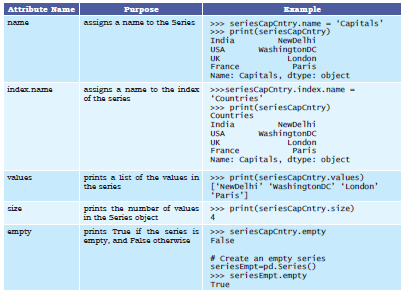
We can access certain properties called attributes of a series by using that property with the series name.Table 2.1 lists some attributes of Pandas series usingseriesCapCntry as an example:

>>> seriesCapCntry

India NewDelhi

USA WashingtonDC

UK London

France Paris

dtype: object

Table 2.1 Attributes of Pandas Series 

2.2.4 Methods of Series

>>> seriesTenTwenty=pd.Series(np.arange( 10,20, 1 ))

>>> print(seriesTenTwenty)

0 10

1 11

2 12

3 13

4 14

5 15

6 16

7 17

8 18

9 19

dtype: int32

2.2.5 Mathematical Operations on Series

We have learnt in Class XI that if we perform basic mathematical operations like addition, subtraction, multiplication, division, etc., on two NumPy arrays, the operation is done on each corresponding pair of elements. Similarly, we can perform mathematical operations on two series in Pandas.

While performing mathematical operations on series, index matching is implemented and all missing values are filled in with NaN by default.

Consider the following series: seriesA and seriesB

for understanding mathematical operations on series in Pandas.

>>> seriesA = pd.Series([1,2,3,4,5], index =

['a', 'b', 'c', 'd', 'e'])

>>> seriesA

a 1

b 2

c 3

d 4

e 5

dtype: int64

>>> seriesB = pd.Series([10,20,-10,-50,100], notes

index = ['z', 'y', 'a', 'c', 'e'])

>>> seriesB

z 10

y 20

a -10

c -50

e 100

dtype: int64

(A) Addition of two Series

It can be done in two ways. In the first method, two series are simply added together, as shown in the following code. Table 2.2 shows the detailed values that were matched while performing the addition. Note here that the output of addition is NaN if one of the elements or both elements have no value.

>>> seriesA + seriesB

a -9.0

b NaN

c -47.0

d NaN

e 105.0

y NaN

z NaN

dtype: float64

Table 2.2 Details of addition of two series index

The second method is applied when we do not want to have NaN values in the output. We can use the series method add() and a parameter fill_value to replace missing value with a specified value. That is, calling seriesA.add(seriesB) is equivalent to calling seriesA+seriesB, but add() allows explicit specification of the fill value for any element in seriesA or seriesB that might be missing, as shown in Table 2.3.

>>> seriesA.add(seriesB, fill_value=0) a -9.0

>>> seriesA.add(seriesB, fill_value=0)

a -9.0

b 2.0

c -47.0

d 4.0

e 105.0

y 20.0

z 10.0

dtype: float64

Table 2.3 Details of addition of two series using add() method

Note that Table 2.2 shows the changes in the series elements and corresponding output without replacing the missing values, while Table 2.3 shows the changes in the series elements and corresponding output after replacing missing values by 0. Just like addition, subtraction, multiplication and division can also be done using corresponding mathematical operators or explicitly calling of the appropriate method.

(B) Subtraction of two Series

Again, it can be done in two different ways, as shown in the following examples: 

>>> seriesA – seriesB #using subtraction operator

a 11.0

b NaN

c 53.0

d NaN

e -95.0

y NaN

z NaN

dtype: float64

Let us now replace the missing values with 1000 before subtracting seriesB from seriesA using explicit subtraction method sub().

>>> seriesA.sub(seriesB, fill_value=1000)

# using fill value 1000 while making explicit

# call of the method”

a 11.0

b -998.0

c 53.0

d -996.0

e -95.0

y 980.0

z 990.0

dtype: float64

(C) Multiplication of two Series

Again, it can be done in two different ways, as shown in the following examples:

>>>seriesA * seriesB #using multiplication operator 

a -10.0

b NaN

c -150.0

d NaN

e 500.0

y NaN

z NaN

dtype: float64

Let us now replace the missing values with 0 before multiplication of seriesB with seriesA using explicit multiplication method mul().

>>> seriesA.mul(seriesB, fill_value=0)

# using fill value 0 while making

#explicit call of the method

a -10.0

b 0.0

c -150.0

d 0.0

e 500.0

y 0.0

z 0.0

dtype: float64

(D) Division of two Series

Again, it can be done in two different ways, as shown in the following examples:

>>> seriesA/seriesB # using division operator

a -0.10

b NaN

c -0.06

d NaN

e 0.05

y NaN

z NaN

dtype: float64

Let us now replace the missing values with 0 before

dividing seriesA by seriesB using explicit division

method div().

# using fill value 0 while making explicit

# call of the method

a -0.10

b inf

c -0.06

d inf

e 0.05

y 0.00

z 0.00

dtype: float64

2.3 DATAFRAME

Sometimes we need to work on multiple columns at a time, i.e., we need to process the tabular data. For example, the result of a class, items in a restaurant’s menu, reservation chart of a train, etc. Pandas store such tabular data using a DataFrame. A DataFrame is a two-dimensional labelled data structure like a table of MySQL. It contains rows and columns, and therefore has both a row and column index. Each column can have a different type of value such as numeric, string, boolean, etc., as in tables of a database.

Column Indexes

2.3.1 Creation of DataFrame

There are a number of ways to create a DataFrame.

Some of them are listed in this section.

(A) Creation of an empty DataFrame

An empty DataFrame can be created as follows: 

>>> import pandas as pd

>>> dFrameEmt = pd.DataFrame()

>>> dFrameEmt

Empty DataFrame

Columns: []

Index: []

(B) Creation of DataFrame from NumPy ndarrays

Consider the following three NumPy ndarrays. Let us create a simple DataFrame without any column labels, using a single ndarray:

>>> import numpy as np

>>> array1 = np.array([10,20,30])

>>> array2 = np.array([100,200,300])

>>> array3 = np.array([-10,-20,-30, -40])

>>> dFrame4 = pd.DataFrame(array1)

>>> dFrame4

0

0 10

1 20

2 30

We can create a DataFrame using more than one ndarrays, as shown in the following example:

>>> dFrame5 = pd.DataFrame([array1, array3, array2], columns=[ 'A', 'B', 'C', 'D'])

>>> dFrame5

>>> dFrame5

A  B   C    D

0 10 20 30 NaN

1 -10 -20 -30 -40.0

2 100 200 300 NaN

(C) Creation of DataFrame from List of Dictionaries

We can create DataFrame from a list of Dictionaries, for example:

# Create list of dictionaries

>>> listDict = [{'a':10, 'b':20}, {'a':5,'b':10, 'c':20}]

>>> dFrameListDict = pd.DataFrame(listDict)

>>> dFrameListDict

a b c

0 10 20 NaN

1 5 10 20.0

Here, the dictionary keys are taken as column labels, and the values corresponding to each key are taken as rows. There will be as many rows as the number of dictionaries present in the list. In the above example there are two dictionaries in the list. So, the DataFrame consists of two rows. Number of columns in a DataFrame is equal to the maximum number of keys in any dictionary of the list. Hence, there are three columns as the second dictionary has three elements.

Also, note that NaN (Not a Number) is inserted if a corresponding value for a column is missing.

(D) Creation of DataFrame from Dictionary of Lists

DataFrames can also be created from a dictionary of lists. Consider the following dictionary consisting of the keys ‘State’, ‘GArea’ (geographical area) and ‘VDF’ (very dense forest) and the corresponding values as list.

>>> dictForest = {'State': ['Assam', 'Delhi','Kerala'],

'GArea': [78438, 1483, 38852] ,

'VDF' : [2797, 6.72,1663]}

>>> dFrameForest= pd.DataFrame(dictForest)

>>> dFrameForest

State GArea VDF

0 Assam 78438 2797.00

1 Delhi 1483 6.72

2 Kerala 38852 1663.00

Note that dictionary keys become column labels by default in a DataFrame, and the lists become the rows.

Thus, a DataFrame can be thought of as a dictionary of lists or a dictionary of series.

We can change the sequence of columns in a DataFrame. This can be done by assigning a particular sequence of the dictionary keys as columns parameter, for example:

>>> dFrameForest1 = pd.DataFrame(dictForest, columns = ['State','VDF', 'GArea'])

>>> dFrameForest1

State VDF GArea

0 Assam 2797.00 78438

1 Delhi 6.72 1483

2 Kerala 1663.00 38852

In the output, VDF is now displayed as the middle column instead of last.

(E) Creation of DataFrame from Series

Consider the following three Series: seriesA = pd.Series([1,2,3,4,5],

index = ['a', 'b', 'c', 'd', 'e']) seriesB = pd.Series ([1000,2000,-1000,-5000,1000], index = ['a', 'b', 'c', 'd', 'e'])

seriesC = pd.Series([10,20,-10,-50,100],

index = ['z', 'y', 'a', 'c', 'e'])

 We can create a DataFrame using a single series as shown below:

>>> dFrame6 = pd.DataFrame(seriesA)

>>> dFrame6

0

a 1

b 2

c 3

d 4

e 5

Here, the DataFrame dFrame6 has as many numbers of rows as the numbers of elements in the series, but has only one column. To create a DataFrame using more than one series, we need to pass multiple series in the list as shown below:

>>> dFrame7 = pd.DataFrame([seriesA, seriesB])

>>> dFrame7

a b c d e

0 1 2 3 4 5

1 1000 2000 -1000 -5000 1000

Observe that the labels in the series object become the column names in the DataFrame object and each series becomes a row in the DataFrame. Now look at the following example:

>>> dFrame8 = pd.DataFrame([seriesA, seriesC])

>>> dFrame8

a b c d e z y 0 1.0 2.0 3.0 4.0 5.0 NaN NaN

1 -10.0 NaN -50.0 NaN 100.0 10.0 20.0

Here, different series do not have the same set of labels. But, the number of columns in a DataFrame equals to distinct labels in all the series. So, if a particular series does not have a corresponding value for a label, NaN is inserted in the DataFrame column.

(F) Creation of DataFrame from Dictionary of Series

A dictionary of series can also be used to create a DataFrame. For example, ResultSheet is a dictionary of series containing marks of 5 students in three subjects.

The names of the students are the keys to the dictionary, and the index values of the series are the subject names as shown below:

>>> ResultSheet={

'Arnab': pd.Series([90, 91, 97],

index=['Maths','Science','Hindi']),

'Ramit': pd.Series([92, 81, 96],

index=['Maths','Science','Hindi']),

'Samridhi': pd.Series([89, 91, 88], index=['Maths','Science','Hindi']),

'Riya': pd.Series([81, 71, 67],

index=['Maths','Science','Hindi']),

'Mallika': pd.Series([94, 95, 99], index=['Maths','Science','Hindi'])}

>>> ResultDF = pd.DataFrame(ResultSheet)

>>> ResultDF

Arnab Ramit Samridhi Riya Mallika

Maths 90 92 89 81 94

ResultDF. Are they the

Science 91 81 91 71 95

Hindi 97 96 88 67 99

The following output shows that every column in the DataFrame is a Series:

>>> type(ResultDF.Arnab)

<class 'pandas.core.series.Series'> When a DataFrame is created from a Dictionary of Series, the resulting index or row labels are a union of all series indexes used to create the DataFrame. For example: dictForUnion = { 'Series1' :

pd.Series([1,2,3,4,5],

index = ['a', 'b', 'c', 'd', 'e']) ,

'Series2' :

pd.Series([10,20,-10,-50,100],

index = ['z', 'y', 'a', 'c', 'e']),

'Series3' :

pd.Series([10,20,-10,-50,100],

index = ['z', 'y', 'a', 'c', 'e']) }

>>> dFrameUnion = pd.DataFrame(dictForUnion)

>>> dFrameUnion

Series1 Series2 Series3

a 1.0 -10.0 -10.0

b 2.0 NaN NaN

c 3.0 -50.0 -50.0

d 4.0 NaN NaN

e 5.0 100.0 100.0

y NaN 20.0 20.0

z NaN 10.0 10.0

2.3.2 Operations on rows and columns in DataFrames

We can perform some basic operations on rows and columns of a DataFrame like selection, deletion, addition, and renaming, as discussed in this section.

(A) Adding a New Column to a DataFrame

We can easily add a new column to a DataFrame. Let us consider the DataFrame ResultDF defined earlier. In order to add a new column for another student ‘Preeti’, we can write the following statement:

>>> ResultDF['Preeti']=[89,78,76]

>>> ResultDF

Arnab Ramit Samridhi Riya Mallika Preeti 

Maths 90 92 89 81 94 89

Science 91 81 91 71 95 78

Hindi 97 96 88 67 99 76

Assigning values to a new column label that does not exist will create a new column at the end. If the column already exists in the DataFrame then the assignment statement will update the values of the already existing column, for example:

>>> ResultDF['Ramit']=[99, 98, 78]

>>> ResultDF

Arnab Ramit Samridhi Riya Mallika Preeti 

Maths 90 99 89 81 94 89

Science 91 98 91 71 95 78

Hindi 97 78 88 67 99 76

We can also change data of an entire column to a particular value in a DataFrame. For example, the following statement sets marks=90 for all subjects for the column name 'Arnab':

>>> ResultDF['Arnab']=90

>>> ResultDF

Arnab Ramit Samridhi Riya Mallika Preeti 

Maths 90 99 89 81 94 89

Science 90 98 91 71 95 78

Hindi 90 78 88 67 99 76

(B) Adding a New Row to a DataFrame

We can add a new row to a DataFrame using the DataFrame.loc[ ] method. Consider the DataFrame ResultDF that has three rows for the three subjects – Maths, Science and Hindi. Suppose, we need to add the marks for English subject in ResultDF, we can use the following statement:

>>> ResultDF

Arnab Ramit Samridhi Riya Mallika Preeti 

Maths 90 92 89 81 94 89

Science 91 81 91 71 95 78

Hindi 97 96 88 67 99 76

>>> ResultDF.loc['English'] = [85, 86, 83, 80, 90, 89]

>>> ResultDF

Arnab Ramit Samridhi Riya Mallika Preeti 

Maths 90 92 89 81 94 89

Science 91 81 91 71 95 78

Hindi 97 96 88 67 99 76

English 85 86 83 80 90 89

We cannot use this method to add a row of data with already existing (duplicate) index value (label). In such case, a row with this index label will be updated, for example:

>>> ResultDF.loc['English'] = [95, 86, 95, 80, 95,99]

>>> ResultDF

Arnab Ramit Samridhi Riya Mallika Preeti 

Maths 90 92 89 81 94 89

Science 91 81 91 71 95 78

Hindi 97 96 88 67 99 76

English 95 86 95 80 95 99

DataFRame.loc[] method can also be used to change the data values of a row to a particular value. For example, the following statement sets marks in 'Maths'

for all columns to 0:

>>> ResultDF.loc['Maths']=0

>>> ResultDF

Arnab Ramit Samridhi Riya Mallika Preeti 

Maths 0 0 0 0 0 0

Science 91 81 91 71 95 78

Hindi 97 96 88 67 99 76

English 95 86 95 80 95 99

If we try to add a row with lesser values than the number of columns in the DataFrame, it results in a ValueError, with the error message: ValueError: Cannot set a row with mismatched columns.

Similarly, if we try to add a column with lesser values than the number of rows in the DataFrame, it results in a ValueError, with the error message: ValueError: Length of values does not match length of index.

Further, we can set all values of a DataFrame to a particular value, for example:

>>> ResultDF[: ] = 0 # Set all values in ResultDF to 0

>>> ResultDF

Arnab Ramit Samridhi Riya Mallika Preeti 

Maths 0 0 0 0 0 0

Science 0 0 0 0 0 0

Hindi 0 0 0 0 0 0

English 0 0 0 0 0 0

(C) Deleting Rows or Columns from a DataFrame

We can use the DataFrame.drop() method to delete rows and columns from a DataFrame. We need to specify the names of the labels to be dropped and the axis from which they need to be dropped. To delete a row, the parameter axis is assigned the value 0 and for deleting a column,the parameter axis is assigned the value 1.

Consider the following DataFrame:

>>> ResultDF

Arnab Ramit Samridhi Riya Mallika 

Maths 90 92 89 81 94

Science 91 81 91 71 95

Hindi 97 96 88 67 99

English 95 86 95 80 95

The following example shows how to delete the row with label 'Science':

>>> ResultDF = ResultDF.drop('Science', axis=0)

>>> ResultDF

Arnab Ramit Samridhi Riya Mallika 

Maths 90 92 89 81 94

Hindi 97 96 88 67 99

English 95 86 95 80 95

The following example shows how to delete the columns having labels 'Samridhi', 'Ramit' and 'Riya':

>>> ResultDF = ResultDF.drop(['Samridhi','Rami t','Riya'], axis=1)

>>> ResultDF

Arnab Mallika

Maths 90 94

Hindi 97 99

English 95 95

If the DataFrame has more than one row with the same label, the DataFrame.drop() method will delete all the matching rows from it. For example, consider the following DataFrame:

>>> ResultDF

Arnab Ramit Samridhi Riya Mallika 

Maths 90 92 89 81 94

Science 91 81 91 71 95

Hindi 97 96 88 67 99

Hindi 97 89 78 60 45

To remove the duplicate rows labelled ‘Hindi’, we need to write the following statement:

>>> ResultDF= ResultDF.drop('Hindi', axis=0)

>>> ResultDF

Arnab Ramit Samridhi Riya Mallika 

Maths 90 92 89 81 94

Science 91 81 91 71 95

(D) Renaming Row Labels of a DataFrame

We can change the labels of rows and columns in a DataFrame using the DataFrame.rename() method.

Consider the following DataFrame. To rename the row indices Maths to sub1, Science to sub2, Hindi to sub3 and English to sub4 we can write the following statement:

>>> ResultDF

Arnab Ramit Samridhi Riya Mallika 

Maths 90 92 89 81 94

Science 91 81 91 71 95

English 97 96 88 67 99

Hindi 97 89 78 60 45

>>> ResultDF=ResultDF.rename({'Maths':'Sub1', What if in the rename

‘Science':'Sub2','English':'Sub3', function we pass a

'Hindi':'Sub4'}, axis='index')

value for a row label

>>> print(ResultDF)

that does not exist?

Arnab Ramit Samridhi Riya Mallika 

Sub1 90 92 89 81 94

Sub2 91 81 91 71 95

Sub3 97 96 88 67 99

Sub4 97 89 78 60 45

The parameter axis='index' is used to specify that the row label is to be changed. If no new label is passed corresponding to an existing label, the existing row label is left as it is, for example:

>>> ResultDF=ResultDF.rename({'Maths':'Sub1',‘Science':'Sub2','Hindi':'Sub4'}, axis='index')

>>> print(ResultDF)

Arnab Ramit Samridhi Riya Mallika 

Sub1 90 92 89 81 94

Sub2 91 81 91 71 95

English 97 96 88 67 99

Sub4 97 89 78 60 45

(E) Renaming Column Labels of a DataFrame

To alter the column names of ResultDF we can again use the rename() method, as shown below. The parameter axis='columns' implies we want to change the column labels:

>>> ResultDF=ResultDF.rename({'Arnab':'Student1','Ramit':'Student2','

Samridhi':'Student3','Mallika':'Student4'},axis='columns')

>>> print(RsultDF)

Student1 Student2 Student3 Riya Student4

Maths 90 92 89 81 94

Science 91 81 91 71 95

English 97 96 88 67 99

Hindi 97 89 78 60 45

Note that the column Riya remains unchanged since we did not pass any new label.

2.3.3 Accessing DataFrames Element through Indexing

Data elements in a DataFrame can be accessed using indexing.There are two ways of indexing Dataframes : Label based indexing and Boolean Indexing.

(A) Label Based Indexing

There are several methods in Pandas to implement label based indexing. DataFrame.loc[ ] is an important method that is used for label based indexing with DataFrames.

Let us continue to use the ResultDF created earlier.

As shown in the following example, a single row label returns the row as a Series.

>>> ResultDF

Arnab Ramit Samridhi Riya Mallika 

Maths 90 92 89 81 94

Science 91 81 91 71 95

Hindi 97 96 88 67 99

>>> ResultDF.loc['Science']

Arnab 91

Ramit 81

Samridhi 91

Riya 71

Mallika 95

Name: Science, dtype: int64

Also, note that when the row label is passed as an integer value, it is interpreted as a label of the index and not as an integer position along the index, for example:

>>> dFrame10Multiples = pd.DataFrame([10,20,30,40,50])

>>> dFrame10Multiples.loc[2]

0 30

Name: 2, dtype: int64

When a single column label is passed, it returns the column as a Series.

>>> ResultDF.loc[:,'Arnab']

Maths 90

Science 91

Hindi 97

Name: Arnab, dtype: int64

Also, we can obtain the same result that is the marks of ‘Arnab’ in all the subjects by using the command:

>>> print(df['Arnab'])

Maths 56

Science 91

English

97 Hindi 97

Name: Arnab, dtype: int64

To read more than one row from a DataFrame, a list of row labels is used as shown below. Note that using [[]]

returns a DataFrame.

>>> ResultDF.loc[['Science', 'Hindi']]

Arnab Ramit Samridhi Riya Mallika 

Science 91 81 91 71 95

Hindi 97 96 88 67 99

(B) Boolean Indexing

Boolean means a binary variable that can represent either of the two states - True (indicated by 1) or False (indicated by 0). In Boolean indexing, we can select the subsets of data based on the actual values in the DataFrame rather than their row/column labels. Thus, we can use conditions on column names to filter data values. Consider the DataFrame ResultDF, the following statement displays True or False depending on whether the data value satisfies the given condition or not.

>>> ResultDF.loc['Maths'] > 90

Arnab False

Ramit True

Samridhi False

Riya False

Mallika True

Name: Maths, dtype: bool

To check in which subjects ‘Arnab’ has scored more than 90, we can write:

>>> ResultDF.loc[:,‘Arnab’]>90

Maths False

Science True

Hindi True

Name: Arnab, dtype: bool

2.3.4 Accessing DataFrames Element through Slicing 

We can use slicing to select a subset of rows and/or columns from a DataFrame. To retrieve a set of rows, 

slicing can be used with row labels. For example:

>>> ResultDF.loc['Maths': 'Science']

Arnab Ramit Samridhi Riya Mallika 

Maths 90 92 89 81 94

Science 91 81 91 71 95

Here, the rows with labels Maths and Science are displayed. Note that in DataFrames slicing is inclusive of the end values. We may use a slice of labels with a column name to access values of those rows in that column only. For example, the following statement displays the rows with label Maths and Science, and column with label Arnab:

>>> ResultDF.loc['Maths': 'Science', ‘Arnab’]

Maths 90

Science 91

Name: Arnab, dtype: int64

We may use a slice of labels with a slice of column names to access values of those rows and columns:

>>> ResultDF.loc['Maths': 'Science', ‘Arnab’:’Samridhi’]

Arnab Ramit Samridhi

Maths 90 92 89

Science 91 81 91

Alternatively, we may use a slice of labels with a list of column names to access values of those rows and columns:

>>> ResultDF.loc['Maths': 'Science',[‘Arnab’,’Samridhi’]]

Arnab Samridhi

Maths 90 89

Science 91 91

Filtering Rows in DataFrames

In DataFrames, Boolean values like True (1) and False (0) can be associated with indices. They can also be used to filter the records using the DataFrmae.loc[] method.

In order to select or omit particular row(s), we can use a Boolean list specifying ‘True’ for the rows to be shown and ‘False’ for the ones to be omitted in the output. For example, in the following statement, row having index as Science is omitted:

>>> ResultDF.loc[[True, False, True]]

Arnab Ramit Samridhi Riya Mallika 

Maths 90 92 89 81 94

Hindi 97 96 88 67 99

2.3.5 Joining, Merging and Concatenation of DataFrames

(A) Joining

We can use the pandas.DataFrame.append() method to merge two DataFrames. It appends rowsof the second DataFrame at the end of the first DataFrame. Columns not present in the first DataFrame are added as new columns. For example, consider the two DataFrames—

dFrame1 and dFrame2described below. Let us use theappend() method to append dFrame2 to dFrame1:

>>> dFrame1=pd.DataFrame([[1, 2, 3], [4, 5],

[6]], columns=['C1', 'C2', 'C3'], index=['R1',

'R2', 'R3'])

>>> dFrame1

C1 C2 C3

R1 1 2.0 3.0

R2 4 5.0 NaN

R3 6 NaN NaN

>>> dFrame2=pd.DataFrame([[10, 20], [30], [40, 50]], columns=['C2', 'C5'], index=['R4', 'R2',

'R5'])

>>> dFrame2

C2 C5

R4 10 20.0

R2 30 NaN

R5 40 50.0

>>> dFrame1=dFrame1.append(dFrame2)

>>> dFrame1

C1 C2 C3 C5

R1 1.0 2.0 3.0 NaN

R2 4.0 5.0 NaN NaN

R3 6.0 NaN NaN NaN

R4 NaN 10.0 NaN 20.0

R2 NaN 30.0 NaN NaN

R5 NaN 40.0 NaN 50.0

Alternatively, if we append dFrame1 to dFrame2, the rows of dFrame2 precede the rows of dFrame1. To get the column labels appear in sorted order we can set the parameter sort=True. The column labels shall appear in unsorted order when the parameter sort = False.

# append dFrame1 to dFrame2

>>> dFrame2 =dFrame2.append(dFrame1, sort=’True’)

>>> dFrame2

C1 C2 C3 C5

R4 NaN 10.0 NaN 20.0

R2 NaN 30.0 NaN NaN

R5 NaN 40.0 NaN 50.0

R1 1.0 2.0 3.0 NaN

R2 4.0 5.0 NaN NaN

R3 6.0 NaN NaN NaN

# append dFrame1 to dFrame2 with sort=False

>>> dFrame2 = dFrame2.append(dFrame1, sort=’False’)

>>> dFrame2

C2 C5 C1 C3

R4 10.0 20.0 NaN NaN

R2 30.0 NaN NaN NaN

R5 40.0 50.0 NaN NaN

R1 2.0 NaN 1.0 3.0

R2 5.0 NaN 4.0 NaN

R3 NaN NaN 6.0 NaN

The parameter verify_integrity of append()method may be set to True when we want to raise an error if the row labels are duplicate. By default, verify_integrity = False. That is why we could append the duplicate row with label R2 when appending the two DataFrames, as shown above.

The parameter ignore_index of append()method may be set to True, when we do not want to use row index labels. By default, ignore_index = False.

>>> dFrame1 = dFrame1.append(dFrame2, ignore_index=True)

>>> dFrame1

C1 C2 C3 C5

0 1.0 2.0 3.0 NaN

1 4.0 5.0 NaN NaN

2 6.0 NaN NaN NaN

3 NaN 10.0 NaN 20.0

4 NaN 30.0 NaN NaN

5 NaN 40.0 NaN 50.0

The append()method can also be used to append a series or a dictionary to a DataFrame.

2.3.6 Attributes of DataFrames

Like Series, we can access certain properties called attributes of a DataFrame by using that property with the DataFrame name. Table 2.4 lists some attributes of Pandas DataFrame. We are going to use a part of the data from a report called “STATE OF FOREST REPORT 2017”, Published by Forest Survey of India, accessible at http://fsi.nic.in/forest-report-2017, as our example data in this section.

As per this report, the geographical area, the area under very dense forests, the area under moderately dense forests, and the area under open forests (all in sq km), in three States of India - Assam, Delhi and Kerala are as shown in the following DataFrame ForestAreaDF:

>>> ForestArea = {

'Assam' :pd.Series([78438, 2797,

10192, 15116], index = ['GeoArea', 'VeryDense',

'ModeratelyDense', 'OpenForest']),

'Kerala' :pd.Series([ 38852, 1663, 9407, 9251],

index = ['GeoArea' ,'VeryDense',

'ModeratelyDense', 'OpenForest']),

'Delhi' :pd.Series([1483, 6.72, 56.24, 129.45], index = ['GeoArea', 'VeryDense',

'ModeratelyDense', 'OpenForest'])}

>>> ForestAreaDF = pd.DataFrame(ForestArea)

>>> ForestAreaDF

Assam Kerala Delhi

GeoArea 78438 38852 1483.00

VeryDense 2797 1663 6.72

ModeratelyDense 10192 9407 56.24

OpenForest 15116 9251 129.45

Table 2.4 Some Attributes of Pandas DataFrame

2.4 ImPortIng and exPortIng data between csV FILes and dataFrames

We can create a DataFrame by importing data from CSV files where values are separated by commas. Similarly, we can also store or export data in a DataFrame as a.csv file.

2.4.1 Importing a CSV file to a DataFrame

Let us assume that we have the following data in a csv file named ResultData.csv stored in the folder C:/NCERT.

In order to practice the code while we progress, you are suggested to create this csv file using a spreadsheet and save in your computer.

RollNo Name Eco Maths

1 Arnab 18 57

2 Kritika 23 45

3 Divyam 51 37

4 Vivaan 40 60

5 Aaroosh 18 27

We can load the data from the ResultData.csv file into a DataFrame, say marks using Pandas read_csv() function as shown below:

>>> marks = pd.read_csv("C:/NCERT/ResultData.

csv",sep =",", header=0)

>>> marks

RollNo Name Eco Maths

0 1 Arnab 18 57

1 2 Kritika 23 45

2 3 Divyam 51 37

3 4 Vivaan 40 60

4 5 Aaroosh 18 27

• The first parameter to the read_csv() is the name of the comma separated data file along with its path.

• The parameter sep specifies whether the values are separated by comma, semicolon, tab, or any other character. The default value for sepis a space.

• The parameter header specifies the number of the row whose values are to be used as the column names. It also marks the start of the data to be fetched. header=0

implies that column names are inferred from the first line of the file. By default, header=0.

We can exclusively specify column names using the parameter names while creating the DataFrame using the read_csv() function. For example, in the following statement, names parameter is used to specify the labels for columns of the DataFrame marks1:

>>> marks1 = pd.read_csv("C:/NCERT/ResultData1.

csv",sep=",",

names=['RNo','StudentName', 'Sub1',

'Sub2'])

>>> marks1

RNo StudentName Sub1 Sub2

0 1 Arnab 18 57

1 2 Kritika 23 45

2 3 Divyam 51 37

3 4 Vivaan 40 60

4 5 Aaroosh 18 27

2.4.2 Exporting a DataFrame to a CSV file

We can use the to_csv() function to save a DataFrame to a text or csv file. For example, to save the DataFrame ResultDF created in the previous section; we can use the following statement:

>>> ResultDF

Arnab Ramit Samridhi Riya Mallika

Maths 90 92 89 81 94

Science 91 81 91 71 95

Hindi 97 96 88 67 99

>>> ResultDF.to_csv(path_or_buf='C:/NCERT/

resultout.csv', sep=',')

This creates a file by the name resultout.csv in the folder C:/NCERT on the hard disk. When we open this file in any text editor or a spreadsheet, we will find the above data along with the row labels and the column headers, separated by comma.

 In case we do not want the column names to be saved to the file we may use the parameter header=False. Another parameter index=False is used when we do not want the row labels to be written to the file on disk. For

example:

>>> ResultDF.to_csv( 'C:/NCERT/resultonly.txt',

sep = '@', header = False, index= False)

If we open the file resultonly.txt, we will find

the following contents:

90@92@89@81@94

91@81@91@71@95

97@96@88@67@99

2.5 PANDAS SERIES VS NUMPY NDARRAY

Pandas supports non-unique index values. If an operation that does not support duplicate index values is attempted, an exception will be raised at that time.

A basic difference between Series and ndarray is that operations between Series automatically align the data based on the label. Thus, we can write computations without considering whether all Series involved have the same label or not.

The result of an operation between unaligned Series (i.e. where the corresponding labels of the series are not the same or are not in the same order) will have the union of the indexes involved. If a label is not found in one Series or the other, the result will be marked as missing NaN. Being able to write code without doing any explicit data alignment grants immense freedom and flexibility in interactive data analysis and research.

Table 2.5 Difference between Pandas Series and NumPy Arrays