Table of Contents

Chapter 15
Probability
It is remarkable that a science, which began with the consideration of games of chance, should be elevated to the rank of the most important subject of human knowledge.
15.1 Introduction
In everyday life, we come across statements such as
(1) It will probably rain today.
(2) I doubt that he will pass the test.
(3) Most probably, Kavita will stand first in the annual examination.
(4) Chances are high that the prices of diesel will go up.
(5) There is a 50-50 chance of India winning a toss in today’s match.
The words ‘probably’, ‘doubt’, ‘most probably’, ‘chances’, etc., used in the statements above involve an element of uncertainty. For example, in (1), ‘probably rain’ will mean it may rain or may not rain today. We are predicting rain today based on our past experience when it rained under similar conditions. Similar predictions are also made in other cases listed in (2) to (5).
The uncertainty of ‘probably’ etc can be measured numerically by means of ‘probability’ in many cases.
Though probability started with gambling, it has been used extensively in the fields of Physical Sciences, Commerce, Biological Sciences, Medical Sciences, Weather Forecasting, etc.
15.2 Probability – an Experimental Approach
In earlier classes, you have had a glimpse of probability when you performed experiments like tossing of coins, throwing of dice, etc., and observed their outcomes. You will now learn to measure the chance of occurrence of a particular outcome in an experiment.
Blaise Pascal(1623–1662)
Fig. 15.1
The concept of probability developed in a very strange manner.In 1654, a gambler Chevalier de Mere, approached the well-known 17th century French philosopher and mathematician Blaise Pascal regarding certain dice problems. Pascal became interested in these problems, studied them and discussed them with another French mathematician, Pierre de Fermat. Both Pascal and Fermat solved the problems independently. This work was the beginning of Probability Theory.
Pierre de Fermat(1601–1665)
Fig. 15.2
The first book on the subject was written by the Italian mathematician, J.Cardan (1501–1576). The title of the book was ‘Book on Games of Chance’ (Liber de Ludo Aleae), published in 1663. Notable contributions were also made by mathematicians J. Bernoulli (1654–1705), P. Laplace (1749–1827), A.A. Markov (1856–1922) and A.N. Kolmogorov (born 1903).
Activity 1 : (i) Take any coin, toss it ten times and note down the number of times a head and a tail come up. Record your observations in the form of the following table
Table 15.1
| Number of times the coin is tossed | Number of times head comes up | Number of times tail comes up |
|---|---|---|
| 10 | ------ | ----- |
Write down the values of the following fractions:
and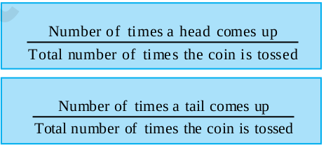
(ii) Toss the coin twenty times and in the same way record your observations as above. Again find the values of the fractions given above for this collection of observations.
(iii) Repeat the same experiment by increasing the number of tosses and record the number of heads and tails. Then find the values of the corresponding fractions.
You will find that as the number of tosses gets larger, the values of the fractions come closer to 0.5. To record what happens in more and more tosses, the following group activity can also be performed:
Activity 2 : Divide the class into groups of 2 or 3 students. Let a student in each group toss a coin 15 times. Another student in each group should record the observations regarding heads and tails. [Note that coins of the same denomination should be used in all the groups. It will be treated as if only one coin has been tossed by all the groups.]
Now, on the blackboard, make a table like Table 15.2. First, Group 1 can write down its observations and calculate the resulting fractions. Then Group 2 can write down its observations, but will calculate the fractions for the combined data of Groups 1 and 2, and so on. (We may call these fractions as cumulative fractions.) We have noted the first three rows ba sed on the observations given by one class of students.
Table 15.2
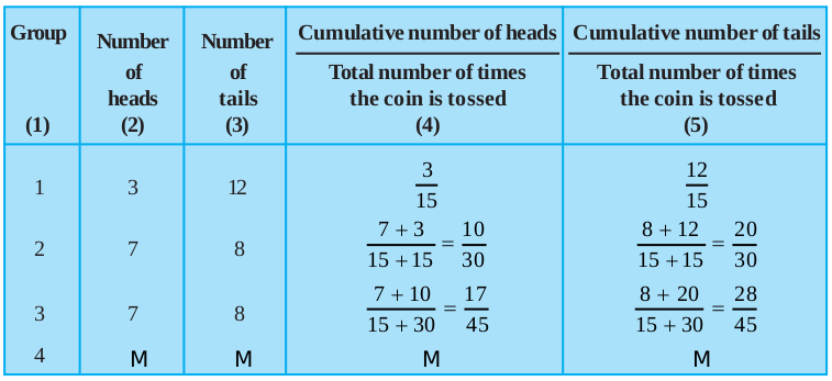
What do you observe in the table? You will find that as the total number of tosses of the coin increases, the values of the fractions in Columns (4) and (5) come nearer and nearer to 0.5.
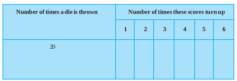
Activity 3 : (i) Throw a die* 20 times and note down the number of times the numbers 1, 2, 3, 4, 5, 6 come up. Record your observations in the form of a table, as in Table 15.3
*A die is a well balanced cube with its six faces marked with numbers from 1 to 6, one number on one face. Sometimes dots appear in place of numbers.
Table 15.3
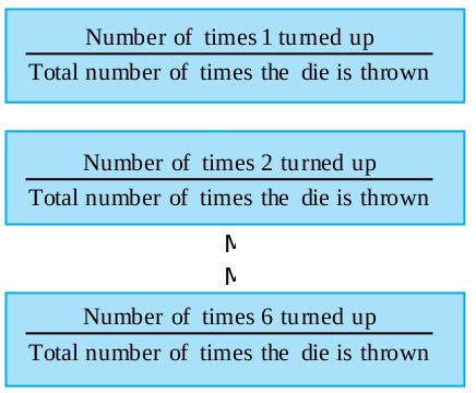
Find the values of the following fractions:
(ii) Now throw the die 40 times, record the observations and calculate the fractions as done in (i).
As the number of throws of the die increases, you will find that the value of each fraction calculated in (i) and (ii) comes closer and closer to  .
.
To see this, you could perform a group activity, as done in Activity 2. Divide the students in your class, into small groups. One student in each group should throw a die ten times. Observations should be noted and cumulative fractions should be calculated.
The values of the fractions for the number 1 can be recorded in Table 15.4. This table can be extended to write down fractions for the other numbers also or other tables of the same kind can be created for the other numbers.
Table 5.4
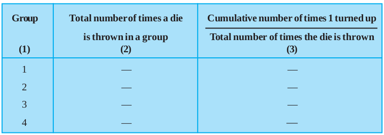
The dice used in all the groups should be almost the same in size and appearence. Then all the throws will be treated as throws of the same die.
What do you observe in these tables?
You will find that as the total number of throws gets larger, the fractions in Column (3) move closer and closer to  .
.
Activity 4 : (i) Toss two coins simultaneously ten times and record your observations in the form of a table as given below:
Table 15.5
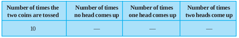
Write down the fractions:
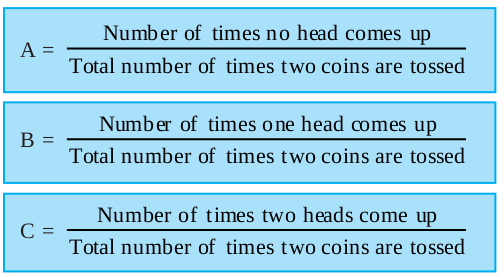
Calculate the values of these fractions.
Now increase the number of tosses (as in Activitiy 2). You will find that the more the number of tosses, the closer are the values of A, B and C to 0.25, 0.5 and 0.25, respectively.
In Activity 1, each toss of a coin is called a trial. Similarly in Activity 3, each throw of a die is a trial, and each simultaneous toss of two coins in Activity 4 is also a trial.
So, a trial is an action which results in one or several outcomes. The possible outcomes in Activity 1 were Head and Tail; whereas in Activity 3, the possible outcomes were 1, 2, 3, 4, 5 and 6.
In Activity 1, the getting of a head in a particular throw is an event with outcome ‘head’. Similarly, getting a tail is an event with outcome ‘tail’. In Activity 2, the getting of a particular number, say 1, is an event with outcome 1.
If our experiment was to throw the die for getting an even number, then the event would consist of three outcomes, namely, 2, 4 and 6.
So, an event for an experiment is the collection of some outcomes of the experiment. In Class X, you will study a more formal definition of an event.
So, can you now tell what the events are in Activity 4?
With this background, let us now see what probability is. Based on what we directly observe as the outcomes of our trials, we find the experimental or empirical probability.
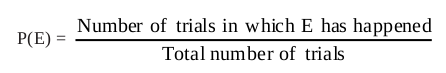
Let n be the total number of trials. The empirical probability P(E) of an event E happening, is given by
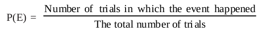
In this chapter, we shall be finding the empirical probability, though we will write ‘probability’ for convenience.
Let us consider some examples.
To start with let us go back to Activity 2, and Table 15.2. In Column (4) of this table, what is the fraction that you calculated? Nothing, but it is the empirical probability of getting a head. Note that this probability kept changing depending on the number of trials and the number of heads obtained in these trials. Similarly, the empirical probability of getting a tail is obtained in Column (5) of Table 15.2. This is  to start with, then it is
  , then
  , and so on.
So, the empirical probability depends on the number of trials undertaken, and the number of times the outcomes you are looking for coming up in these trials.
Activity 5 : Before going further, look at the tables you drew up while doing Activity 3. Find the probabilities of getting a 3 when throwing a die a certain number of times. Also, show how it changes as the number of trials increases.
Now let us consider some other examples.
Example 1 : A coin is tossed 1000 times with the following frequencies:
Head : 455, Tail : 545
Compute the probability for each event.
Solution : Since the coin is tossed 1000 times, the total number of trials is 1000. Let us call the events of getting a head and of getting a tail as E and F, respectively. Then, the number of times E happens, i.e., the number of times a head come up, is 455.
So, the probability of E =
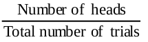
i.e., 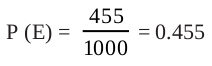
Similarly, the probability of the event of getting a tail 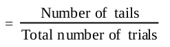
i.e.,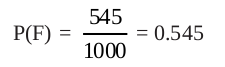
Note that in the example above, P(E) + P(F) = 0.455 + 0.545 = 1, and E and F are the only two possible outcomes of each trial.
Example 2 : Two coins are tossed simultaneously 500 times, and we get
Two heads : 105 times
One head : 275 times
No head : 120 times
Find the probability of occurrence of each of these events.
Solution : Let us denote the events of getting two heads, one head and no head by E1, E2 and E3, respectively. So,
P(E1) =  = 0.21
P(E2) =  = 0.55
P(E3) =  = 0.24
Observe that P(E1) + P(E2) + P(E3) = 1. Also E1, E2 and E3 cover all the outcomes of a trial.
Example 3 : A die is thrown 1000 times with the frequencies for the outcomes 1, 2, 3, 4, 5 and 6 as given in the following table :
Table 15.6
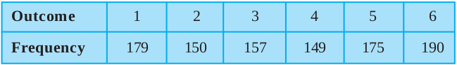
Find the probability of getting each outcome.
Solution : Let Ei denote the event of getting the outcome i, where i = 1, 2, 3, 4, 5, 6. Then
Probability of the outcome 1 =
=  = 0.179
Similarly, P(E2) =  = 0.15, P(E3) =
  = 0.157,
P(E4) =  = 0.149, P(E5) =
  = 0.175
and P(E6) =  = 0.19.
Note that P(E1) + P(E2) + P(E3) + P(E4) + P(E5) + P(E6) = 1
Also note that:
(i) The probability of each event lies between 0 and 1.
(ii) The sum of all the probabilities is 1.
(iii) E1, E2, . . ., E6 cover all the possible outcomes of a trial.
Example 4 : On one page of a telephone directory, there were 200 telephone numbers. The frequency distribution of their unit place digit (for example, in the number 25828573, the unit place digit is 3) is given in Table 15.7 :
Table 15.7
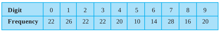
Without looking at the page, the pencil is placed on one of these numbers, i.e., the number is chosen at random. What is the probability that the digit in its unit place is 6?
Solution : The probability of digit 6 being in the unit place
= 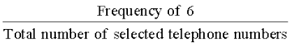
=  = 0.07
You can similarly obtain the empirical probabilities of the occurrence of the numbers having the other digits in the unit place.
Example 5 : The record of a weather station shows that out of the past 250 consecutive days, its weather forecasts were correct 175 times.
(i) What is the probability that on a given day it was correct?
(ii) What is the probability that it was not correct on a given day?
Solution : The total number of days for which the record is available = 250
(i) P(the forecast was correct on a given day)=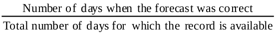
=  = 0.7
= 0.7
(ii) The number of days when the forecast was not correct = 250 – 175 = 75
So, P(the forecast was not correct on a given day) =  = 0.3
= 0.3
Notice that:
P(forecast was correct on a given day) + P(forecast was not correct on a given day)
= 0.7 + 0.3 = 1
Example 6 : A tyre manufacturing company kept a record of the distance covered before a tyre needed to be replaced. The table shows the results of 1000 cases.
Table 15.8
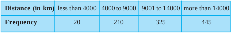
If you buy a tyre of this company, what is the probability that :
(i) it will need to be replaced before it has covered 4000 km?
(ii) it will last more than 9000 km?
(iii) it will need to be replaced after it has covered somewhere between 4000 km and 14000 km?
Solution : (i) The total number of trials = 1000.
The frequency of a tyre that needs to be replaced before it covers 4000 km is 20.
So, P(tyre to be replaced before it covers 4000 km) =  = 0.02
(ii) The frequency of a tyre that will last more than 9000 km is 325 + 445 = 770
So, P(tyre will last more than 9000 km) =  = 0.77
(iii) The frequency of a tyre that requires replacement between 4000 km and
14000 km is 210 + 325 = 535.
So, P(tyre requiring replacement between 4000 km and 14000 km) =  = 0.535
Example 7 : The percentage of marks obtained by a student in the monthly unit tests are given below:
Table 5.9
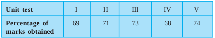
Based on this data, find the probability that the student gets more than 70% marks in a unit test.
Solution : The total number of unit tests held is 5.
The number of unit tests in which the student obtained more than 70% marks is 3.
So, P(scoring more than 70% marks) =  = 0.6
= 0.6
Example 8 : An insurance company selected 2000 drivers at random (i.e., without any preference of one driver over another) in a particular city to find a relationship between age and accidents. The data obtained are given in the following table:
Table 15.10
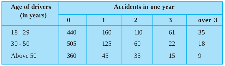
Find the probabilities of the following events for a driver chosen at random from the city:
(i) being 18-29 years of age and having exactly 3 accidents in one year.
(ii) being 30-50 years of age and having one or more accidents in a year.
(iii) having no accidents in one year.
Solution : Total number of drivers = 2000.
(i) The number of drivers who are 18-29 years old and have exactly 3 accidents in one year is 61.
So, P (driver is 18-29 years old with exactly 3 accidents) = 
= 0.0305 ≈ 0.031
(ii) The number of drivers 30-50 years of age and having one or more accidents in one year = 125 + 60 + 22 + 18 = 225
So, P(driver is 30-50 years of age and having one or more accidents)
=  = 0.1125 ≈ 0.113
(iii) The number of drivers having no accidents in one year = 440 + 505 + 360
= 1305
Therefore, P(drivers with no accident) =  = 0.653
Example 9 : Consider the frequency distribution table (Table 14.3, Example 4, Chapter 14), which gives the weights of 38 students of a class.
(i) Find the probability that the weight of a student in the class lies in the interval
46-50 kg.
(ii) Give two events in this context, one having probability 0 and the other having probability 1.
Solution : (i) The total number of students is 38, and the number of students with weight in the interval 46 - 50 kg is 3.
So, P(weight of a student is in the interval 46 - 50 kg) =  = 0.079
(ii) For instance, consider the event that a student weighs 30 kg. Since no student has this weight, the probability of occurrence of this event is 0. Similarly, the probability of a student weighing more than 30 kg is  = 1.
= 1.
Example 10 : Fifty seeds were selected at random from each of 5 bags of seeds, and were kept under standardised conditions favourable to germination. After 20 days, the number of seeds which had germinated in each collection were counted and recorded as follows:
Table 5.11
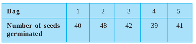
What is the probability of germination of
(i) more than 40 seeds in a bag?
(ii) 49 seeds in a bag?
(iii) more that 35 seeds in a bag?
Solution : Total number of bags is 5.
(i) Number of bags in which more than 40 seeds germinated out of 50 seeds is 3.
P(germination of more than 40 seeds in a bag) =  = 0.6
= 0.6
(ii) Number of bags in which 49 seeds germinated = 0.
P(germination of 49 seeds in a bag) =  = 0.
= 0.
(iii) Number of bags in which more than 35 seeds germinated = 5.
So, the required probability = = 1.
= 1.
Remark : In all the examples above, you would have noted that the probability of an event can be any fraction from 0 to 1.
Exercise 15.1
1. In a cricket match, a batswoman hits a boundary 6 times out of 30 balls she plays. Find the probability that she did not hit a boundary.
2. 1500 families with 2 children were selected randomly, and the following data were recorded:
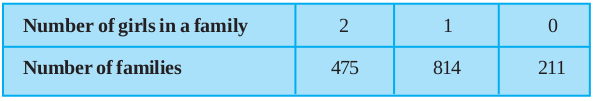
Compute the probability of a family, chosen at random, having
(i) 2 girls (ii) 1 girl (iii) No girl
Also check whether the sum of these probabilities is 1.
3. Refer to Example 5, Section 14.4, Chapter 14. Find the probability that a student of the class was born in August.
4. Three coins are tossed simultaneously 200 times with the following frequencies of different outcomes: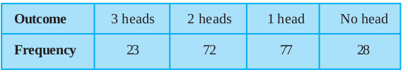
If the three coins are simultaneously tossed again, compute the probability of 2 heads coming up.
5. An organisation selected 2400 families at random and surveyed them to determine a relationship between income level and the number of vehicles in a family. The information gathered is listed in the table below:
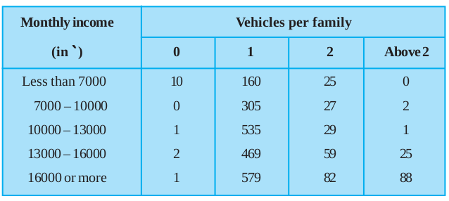
Suppose a family is chosen. Find the probability that the family chosen is
(i) earning Rs 10000 – 13000 per month and owning exactly 2 vehicles.
(ii) earning Rs 16000 or more per month and owning exactly 1 vehicle.
(iii) earning less than Rs 7000 per month and does not own any vehicle.
(iv) earning Rs 13000 – 16000 per month and owning more than 2 vehicles.
(v) owning not more than 1 vehicle.
6. Refer to Table 14.7, Chapter 14.
(i) Find the probability that a student obtained less than 20% in the mathematics test.
(ii) Find the probability that a student obtained marks 60 or above.
7. To know the opinion of the students about the subject statistics, a survey of 200 students was conducted. The data is recorded in the following table.
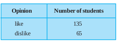
Find the probability that a student chosen at random
(i) likes statistics, (ii) does not like it.
8. Refer to Q.2, Exercise 14.2. What is the empirical probability that an engineer lives:
(i) less than 7 km from her place of work?
(ii) more than or equal to 7 km from her place of work?
(iii) within  km from her place of work?
9.Activity : Note the frequency of two-wheelers, three-wheelers and four-wheelers going past during a time interval, in front of your school gate. Find the probability that any one vehicle out of the total vehicles you have observed is a two-wheeler.
10.Activity : Ask all the students in your class to write a 3-digit number. Choose any student from the room at random. What is the probability that the number written by her/him is divisible by 3? Remember that a number is divisible by 3, if the sum of its digits is divisible by 3.
11. Eleven bags of wheat flour, each marked 5 kg, actually contained the following weights of flour (in kg):

Find the probability that any of these bags chosen at random contains more than 5 kg of flour.
12. In Q.5, Exercise 14.2, you were asked to prepare a frequency distribution table, regarding the concentration of sulphur dioxide in the air in parts per million of a certain city for 30 days. Using this table, find the probability of the concentration of sulphur dioxide in the interval 0.12 - 0.16 on any of these days.
13. In Q.1, Exercise 14.2, you were asked to prepare a frequency distribution table regarding the blood groups of 30 students of a class. Use this table to determine the probability that a student of this class, selected at random, has blood group AB.
15.3 Summary
In this chapter, you have studied the following points:
1. An event for an experiment is the collection of some outcomes of the experiment.
2. The empirical (or experimental) probability P(E) of an event E is given by
3. The Probability of an event lies between 0 and 1 (0 and 1 inclusive).