Table of Contents

Chapter 4
Describing Motion Around Us

Everything in nature is in motion, from massive astronomical objects to subatomic particles. We have a wide variety of motion in nature, such as flitting butterflies, slithering snakes, hopping hares, galloping horses, tendrils of climbers twinning around a support, closing of flytraps, dancing dust particles in a sunbeam, smoke particles moving in air, rising and falling of ocean tides, and gathering clouds.
Isn’t motion in nature wonderful? But how do we study the wide variety of complex motions around us? As you have read in the first chapter, to explore a complex phenomenon, scientists first study it in its idealised simplified forms. Such types of motion are linear, circular and oscillatory about which you learnt in earlier grades. In this chapter, you will learn more about linear motion (motion in a straight line) and uniform circular motion.
Earlier, you learnt about some physical quantities, such as distance, time and speed. Now, you will learn about some more physical quantities, such as displacement, average velocity and average acceleration. You will also learn to describe motion not only in words, but also with numbers, equations and graphs.
Think It Over
- How much distance should we maintain from the truck ahead to avoid a collision if it suddenly applies the brakes?
- Does this distance depend upon the speed with which we are moving?
4.1 Motion in a Straight Line
You have learnt that when an object moves in a straight line, its motion is called linear motion. It can also be called motion in a straight line. It is the simplest kind of motion. Have you noticed it around you, such as children in a swimming race, a vertically falling ball, a car moving along a straight stretch of a highway or a train moving on a straight track (Fig. 4.1)?
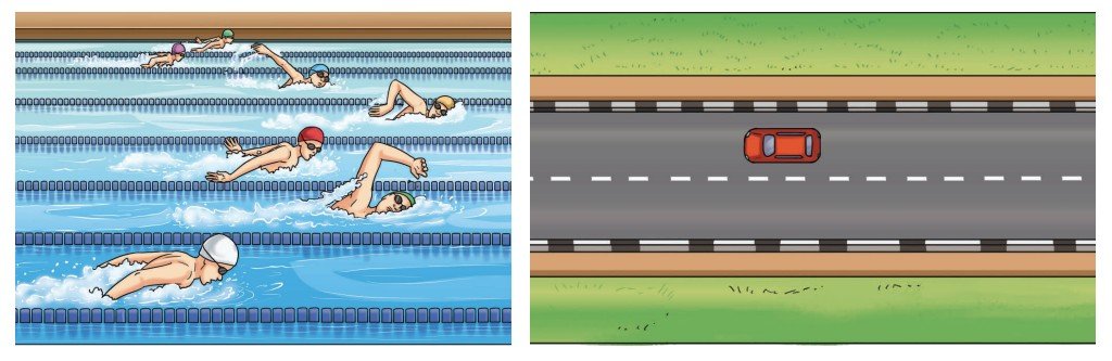
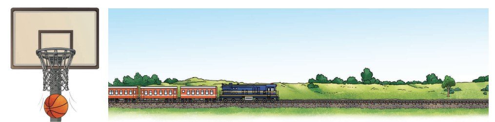
To discuss about the motion of an object, you first need to describe its position at various instants of time.
4.1.1 Describing position
How do we describe the position of an object? For that, as you learnt earlier, we first need to specify a fixed point as the reference point. The distance and direction of the object with respect to the reference point, at any instant of time, describes the position of the object at that instant of time. Note that apart from the distance, we also specify the direction from the reference point in which the object is located to describe its position. But when do we say that an object is in motion? If the position of the object with respect to the reference point changes with time, the object is said to be in motion. On the other hand, the object is said to be at rest if its position with respect to the reference point does not change with time.
Let us take the example of an athlete running on a straight track (Fig. 4.2).
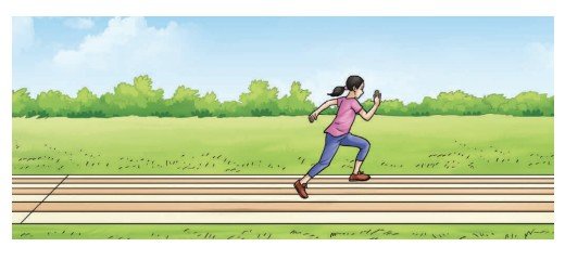
To describe the position of Neena, an athlete, let us take her starting point as the reference point. As shown in Fig. 4.3, let us make a straight line with distances marked on it and mark the reference point on it as the origin ʻOʼ. The athlete starts running from O, and her positions at two instants of time are marked by points B and A.

To describe the position of an object, we also need to specify its direction. For the object moving in a straight line, the object can move only in one of the two directions — forward and backward. Thus, the direction is represented by plus ( ) and minus (–) signs as shown in Fig. 4.3. Positions to the right of the reference point O are generally taken as positive and to the left of O as negative (Fig. 4.3).
Note
4.1.2 Distance travelled and displacement
Suppose an athlete starts running from point O at time t = 0 s, reaches point B at t = 4 s, then reaches point A at t = 10 s, then runs back along the same path till point B reaching there at t = 16 s (Fig. 4.4). How much is the total distance travelled by the athlete between the starting and stopping positions? The total distance travelled is OA + AB = 100 m + 60 m = 160 m.
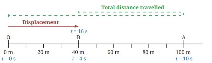
Let us now think about the distance between the starting and the stopping positions of the athlete. It is OB = 40 m, which is different from the total distance travelled by the athlete. So, let us now define another quantity — displacement.
Displacement is the net change in the position of an object between the two given instants of time. A complete description of physical quantities like displacement requires specifying both a direction and its numerical value (with units). The numerical value (with units) of such a physical quantity is called its magnitude. The magnitude of displacement is the distance between the object’s positions at the two instants. The direction of displacement is specified from the position at the first instant towards the position at the second instant. To describe the total distance travelled, only the numerical value (with units) is required, not the direction of motion. The SI unit for both is the metre (m).
For example, in Fig. 4.4, between t = 0 s and t = 16 s, the total distance travelled by the athlete is 160 m, but her displacement is 40 m in the positive direction. We find that between these two instants, the total distance travelled and the magnitude of displacement are not equal. Can these quantities ever be equal?
Ready to Go Beyond
Note
Activity 4.1: Let us analyse
- As shown in Fig. 4.5, a ball is thrown vertically upwards from O. It moves up straight till B and then falls back to O. Can this be considered a motion in a straight line?
- For this motion, fill up the values in Table 4.1.
- Analyse the data filled in Table 4.1 and choose which of the following is true for displacement:
- It is never zero.
- Its magnitude can be greater than the total distance travelled.
- Its magnitude is less than or equal to the total distance travelled.
- Its magnitude is less than the total distance travelled in all cases
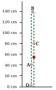
Table 4.1: Distance travelled and displacement of the ball
| S. No. | Position | Total distance travelled by the ball from O till that position | Displace-ment of the ball from O till that position |
|---|---|---|---|
| 1. | O | 0 cm | 0 cm |
| 2. | A | 40 cm | 40 cm in upward direction |
| 3. | B | ||
| 4. | C | ||
| 5. | O |
Pause and Ponder
- In the example of an athlete running back and forth on a straight track (Fig. 4.4), when will the displacement of the athlete be zero? What will be the total distance travelled in that case?
- Fuel used up in a vehicle depends on which of the following? Justify your answer.
- Total distance travelled
- Displacement
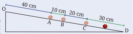
- A ball rolls down an inclined track as shown in Fig. 4.6. Is its motion, a straight line motion? Assuming the starting point of the ball (O) to be the origin, can its motion from O to D be depicted using a horizontal line as shown in Fig. 4.3? Are the values of total distance travelled and magnitude of displacement from O equal or different at positions A, B, C and D?
Motion, i.e., a change in the position of an object, can be described in terms of the total distance travelled by the object and its displacement. But how can you describe how fast or slow an object is moving?
4.1.3 Average speed and average velocity
You have learnt about average speed in an earlier grade. It tells us how fast or slow an object moves. The average speed of an object is the total distance travelled divided by the time interval during which this distance is covered. Thus,
average speed = total distance travelled/time interval (4.1)
Since distance travelled has no direction (but only a numerical value), the average speed, which is calculated from distance travelled, also has no direction but only a numerical value.
If an object moving in a straight line travels equal distances in equal intervals of time (for all possible choices of time intervals), it is said to be in uniform motion in a straight line. In this case, the object moves at a constant speed. On the other hand, if the object travels unequal distances in equal intervals of time, then it is in non-uniform motion in a straight line. In this case, the object moves with increasing speed or decreasing speed, or a combination of both. If the distances travelled in the successive intervals of times are increasing, its speed is increasing.
Indiaʼs Scientific Contributions
Example 4.1: Consider two postmen. They start walking towards each other from a distance of 210 yojanas (Yojana is a unit of distance used in ancient India). One travels 9 yojanas per day and the other covers 5 yojanas per day. Can you determine in how many days they will meet each other?
Answer:
Total of distance covered by each postman in one day = 9 yojanas + 5 yojanas = 14 yojanas.
To meet with each other, the postmen need to cover 210 yojanas together.
Time taken by them to cover 210 yojanas together = 210/14 = 15 days.
So, both postmen will meet each other after 15 days.
(In 15 days, first postman will cover 135 yojanas and the second postman will cover 75 yojanas).
The speed tells us how fast an object is moving but it provides no information about the direction of motion. There are many situations where along with the speed, you also need to know the direction of motion to get a complete picture, particularly in case of complicated real-world motions.
Let us define another physical quantity, average velocity, which describes how fast the position of an object is changing and in which direction.
The average velocity of an object in a time interval is the change in the position (or displacement) divided by the time interval in which the change in position (or displacement) occurs. Thus,
average velocity = change in position/time interval = displacement/time interval (4.2a)
If we represent average velocity by vav , displacement by s and time interval by t, then Eq. (4.2a) can be written as
vav = s/t (4.2b)
To express the average velocity, you need to specify its magnitude as well as the direction. How do we associate direction with velocity when the motion is in a straight line? The direction of the velocity is the same as the direction of displacement and is indicated by a ʻ ʼ or ʻ–ʼ sign.
Note
The SI unit of average speed and average velocity are the same. It is metre per second which is represented by m s–1 or m/s. It is also commonly measured in kilometre per hour (km h–1).
To describe how fast or slow a change in a physical quantity happens, we use the idea of a rate of change. The ratio of change in one quantity to the corresponding change in time is called the rate of change. To calculate average velocity, we find the ratio of change in position to the time taken (Eq. 4.2a). So, we can say that average velocity is the average rate of change of position of an object with respect to time.
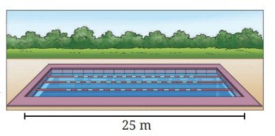
Example 4.2: Sarang takes 50 seconds to swim from one end to the other end and back in the swimming pool shown in Fig. 4.7. Find his average speed and average velocity within the time interval of 50 s.
Answer:
Total distance travelled by Sarang in 50 s = 50 m
displacement of Sarang in 50 s = 0 m
average speed = total distance travelled/time interval = 50 m/50 s = 1 ms-1
average velocity = displacement/time interval = 0 m/50 s = 0 ms-1
During the 50 s time interval, the average speed of Sarang is approximately 1 ms –1 while his average velocity is 0 ms –1.
Pause and Ponder
- During a family road trip, you drive 200 km north in three hours. Afterwards, you drive 200 km south in two hours. Find the average speed and average velocity for your entire trip.
- Under what condition(s) is the
- magnitude of average velocity of an object equal to its average speed?
- magnitude of average velocity of an object zero while its average speed is not zero?
The average velocity of an object over a large time interval may differ from its velocity at a particular instant. Throughout this chapter, we will use the term ‘velocity’ to mean the velocity of an object at a particular instant.
Ready to Go Beyond
The velocity of an object can be constant or it can change with time. How can we express the change in velocity of an object?
Threads of Curiosity
4.1.4 Average acceleration
When you sit in a vehicle and it suddenly moves from rest, you feel a noticeable jolt. Similarly, when the vehicle is in motion and suddenly stops, you experience a jolt. These occurrences capture the feeling of the change in velocity. You can find the change in velocity if you know the velocity at two different instants of time.
Let us now learn another physical quantity, the average acceleration. The average acceleration of an object over a time interval is the change in its velocity divided by the time interval. That is,
average acceleration = change in velocity/time interval (4.3a)
average acceleration = final velocity initial velocity/time interval (4.3b)
If the velocity of an object changes from an initial value u at time t1 to the final value v at time t2, the average acceleration a is,
a = v-u/(t2-t1) (4.3c)
The SI unit of average acceleration is ms–2 or m/s2. Like displacement and velocity, we need to specify the magnitude as well as the direction of acceleration. For motion in a straight line, if the magnitude of velocity is increasing in a given time interval, the average acceleration is in the direction of velocity (Fig. 4.8). Whereas, the average acceleration is opposite to the direction of velocity if the magnitude of velocity is decreasing.
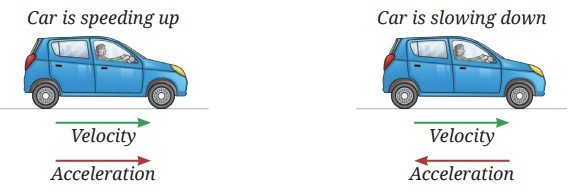
The average acceleration can result from change in the magnitude of velocity or change in its direction, or both. Later in Section 4.4, we will discuss an example of acceleration resulting from only the change of direction of the motion while the speed remains constant.
Activity 4.2: Let us calculate
- The magnitude of average acceleration of cars is generally specified as the time taken by the car to go from 0kmh–1 to 100kmh–1. Look it up on the internet and find this time for various cars, and record those in Table 4.2.
- Calculate the magnitude of average acceleration for each car.
Table 4.2: The magnitude of average acceleration in a time interval
| Car type | Time interval during which the speed goes from 0 to 100 km h–1 | Magnitude of average acceleration (m s–2) |
|---|---|---|
Example 4.3: A bus is moving on a long straight highway (Fig. 4.9) with a velocity of 36 km h–1. The driver presses the accelerator for a time interval of 10 s and velocity of the bus increases to 54 km h–1. For some time, the bus moves at a constant velocity. Then, the driver notices an obstacle on the road ahead and presses the brake. The bus comes to a stop in a time interval of 5 s. Find the average acceleration in the two time intervals, (i) when the accelerator was pressed, and (ii) when the brakes were pressed.

Answer: (i) When the driver presses the accelerator
u = 36 km h–1 = 36 ×1000 m/60×60 s = 10 m s–1, v = 54 km h–1 = 15 m s–1, t = 10 s, a = ?
Using Eq. (4.3c), we obtain the average acceleration
a = 15 m s–1-10 m s–1/10 s = 5 m s–1/10 s = 0.5 m s–2
Since the magnitude of velocity of the bus is increasing, the acceleration is acting in the direction of velocity.
(ii) When the driver presses the brake
u = 54 km h–1 = 15 m s–1, v = 0 m s–1, t = 5 s, a = ?
Using Eq. (4.3c) again, we obtain
a = 0 m s–1-15 m s–1/5 s = -15 m s–1/5 s = -3 m s–1
The minus sign indicates that the acceleration is acting opposite to the direction of velocity (since the magnitude of velocity of the bus is decreasing).
Note
The average acceleration during different time intervals can either be constant or changing. For an object moving in a straight line in the same direction, if the magnitude of its velocity increases or decreases by equal amounts in equal intervals of time (for all possible choices of time intervals), the acceleration of the object is constant.
Note
Example 4.4: As we learnt earlier, when an object is dropped from a height, it takes a straight vertical path downwards before touching the ground. While coming down, the velocity of the object increases as shown in Fig. 4.10 at different instants. Find the magnitude of the average acceleration of the object in every successive interval of a second. Is the average acceleration constant across all intervals? What is the direction of this average acceleration?
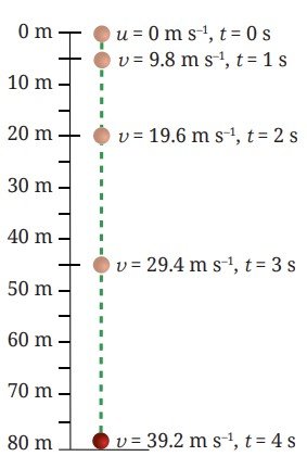
Answer: The magnitude of the average acceleration in every successive interval is
average acceleration between 0 s and 1 s = (9.8-0)ms-1/(1-0)s = 9.8ms-2
average acceleration between 1 s and 2 s = (19.6-9.8)ms-1/(2-1)s = 9.8ms-2
average acceleration between 2 s and 3 s = (29.4-19.6)ms-1/(3-2)s = 9.8ms-2
average acceleration between 3 s and 4 s = (39.2-29.4)ms-1/(4-3)s = 9.8ms-2
We note that the average acceleration is constant and equal to 9.8 m s–2. As the velocity is increasing in the direction of motion, the acceleration is in the direction of motion. This acceleration is called the acceleration due to gravitational force by the Earth and is denoted by g.
Did you notice that in Fig. 4.5, we chose the origin at the ground level while in Fig. 4.10, we chose the origin at the point from where the object is dropped? In this example, we use down side as positive. We can choose the origin and positive direction as per our convenience. However, once chosen, it should not be changed while solving a problem.
Just like we can specify the velocity of an object at an instant, we can specify the acceleration of an object at an instant.
Ready to Go Beyond
4.2 Graphical Representation of Motion
One useful way of representing motion can be a graphical representation. It provides a visual representation of how position, velocity and acceleration change with time. Such graphs help in comparing the motion of two objects, in calculating physical quantities, or in identifying whether the motion is uniform or non-uniform.
As you have learnt in Mathematics, graphs come in various forms, each suited to different types of data representation. To describe motion, we will use graphs to show dependence of one physical quantity, such as position, velocity or acceleration, on another quantity, such as time. Let us learn to plot and interpret line graphs for motion.
Note
4.2.1 Plotting graph
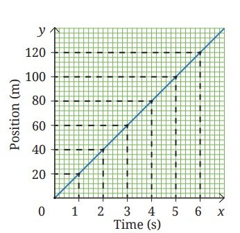
To plot a graph, let us use the data given in Table 4.3 for a vehicle moving on a straight road.
Table 4.3: Positions of vehicle at different instants of time
| Time | 0 s | 1 s | 2 s | 3 s | 4 s | 5 s | 6 s |
| Position | 0 m | 20 m | 40 m | 60 m | 80 m | 100 m | 120 m |
Activity 4.3: Let us plot a graph
- Take a sheet of graph paper. This paper is pre-divided into small squares (Fig. 4.11a), making it easier to plot data accurately.
- On the graph paper, draw two lines perpendicular to each other as shown in Fig. 4.11a. Their point of intersection is known as origin O. Mark the horizontal line as OX. It is known as the x-axis. Similarly, mark the vertical line as OY. It is called the y-axis.
- Refer to Table 4.3. We need to decide which quantity (time or position) to be shown along each axis. For the data we have (Table 4.3), we will show time along the x-axis and position along the y-axis.
- Determine a suitable scale for each quantity to represent it on the graph paper. We need to choose scales that allow us to represent the data effectively and conveniently while utilising the available space. The scale can be
x-axis: 5 divisions = 1 s
y-axis: 5 divisions = 20 m - Use the chosen scale to mark values for time (1 s, 2 s, …) along the x-axis from the origin. Similarly, mark values for position (20 m, 40 m, …) along the y-axis (Fig. 4.11b).
- Begin plotting points on the graph paper to represent each set of time and position values from Table 4.3.
- Table 4.3 shows that at time 0 s, the position is also 0 m. The point corresponding to this set of values on the graph will therefore be the origin itself.
- At 1 s, the position of vehicle is at 20 m. To mark these values, look for the point that represents 1 s on the x-axis. Draw a line parallel to the y-axis at this point. Then, draw a line parallel to the x-axis from the point corresponding to distance 20 m on the y-axis. The point where these two lines intersect represents the position 20 m at time t = 1 s on the graph (Fig. 4.11b).
- Similarly, plot on the graph paper all points corresponding to positions of the vehicle at different instants of time.
- Once all points are plotted, connect them to create the position-time graph for the vehicle’s motion (Fig. 4.11c). It is a straight line for the data given in Table 4.3.
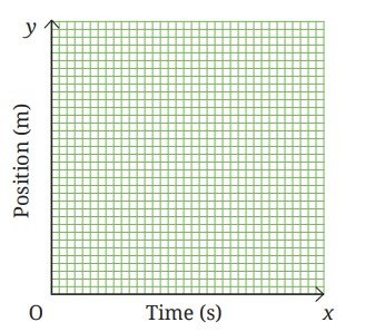
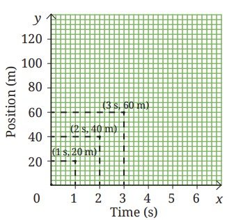
This was an example of plotting a position-time graph. Similar procedure can be used to plot the other graphs which you will be learning ahead.
Ready to Go Beyond
Note
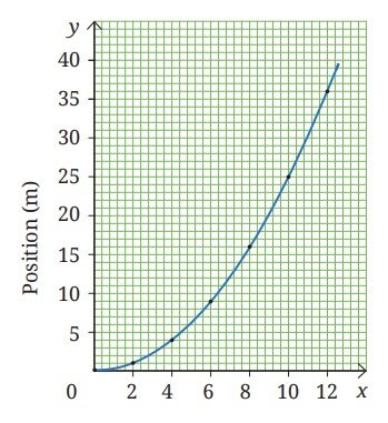
Example 4.5: For a vehicle starting from rest and speeding up, the data for position and time are given in Table 4.4. Plot the position-time graph corresponding to it.
Table 4.4: Positions of vehicle at different instants of time
| Time | Position |
|---|---|
| 0 s | 0 m |
| 2 s | 1 m |
| 4 s | 4 m |
| 6 s | 9 m |
| 8 s | 16 m |
| 10 s | 25 m |
| 12 s | 36 m |
Answer:
Choosing the scale to be
x-axis: 5 divisions = 2 s
y-axis: 5 divisions = 5 m
and following the procedure of Activity 4.3, all points corresponding to positions of the vehicle at different instants of time are marked. Unlike Fig. 4.11c, the points do not fall on a straight line. The points can be joined by a curve as shown in Fig. 4.12.
Now that you know how to plot a graph from the data given for the motion of an object, let us learn to interpret the graphs.
4.2.2 Position-time graphs
The position-time graph represents the motion of object, i.e., the change in its position with time. You have already plotted two position-time graphs (Figs. 4.11c and 4.12). Now, what information can you obtain from these graphs about the motion of the object?
What does the shape of the position-time graph indicate about the nature of motion?
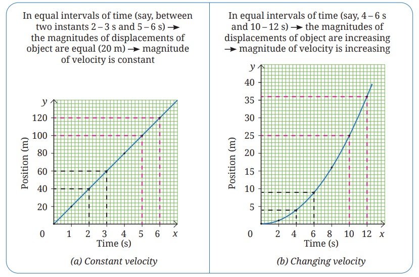
As we can see in Fig. 4.13a, a straight line position-time graph indicates that the object is moving with a constant velocity. On the other hand, a curved position-time graph as in Fig. 4.13b, indicates that the velocity is not constant, and thus, the object is in accelerated motion.
Which physical quantities can be obtained from a position-time graph?
From the position-time graph, you can find the position of an object at each instant of time. Does the graph provide information about any other physical quantity as well? In fact, you can also calculate how fast the position is changing, i.e., the magnitude of velocity of the object. How can you do that?
Activity 4.4: Let us calculate
- In the position-time graph we plotted (Fig. 4.11c), consider a part (say, AB) of the graph as shown in Fig. 4.14. From A, draw a line parallel to x-axis and another line parallel to Y-axis. Repeat the same from B.
- Extend the horizontal line from A and a triangle ABC is formed. What do the sides BC and CA of the triangle represent? BC represents the change in position (s2–s1), and AC represents the change in time (t2–t1).
- As per Eq. (4.2a), by dividing the change in position (BC) by the change in time (CA), you get the average velocity
v = s2–s1/t2–t1 = BC/CA - By extracting values of time t1 and t2, and distances s1 and s2 from the graph, the magnitude of average velocity can be calculated as v = (80 m-40 m)/(4 s-2 s) = 40 m/ 2 s = 20 m s-1
From a position-time graph, by finding the positions of the object at two instants of time, you can calculate the average velocity by using Eq. (4.2a).
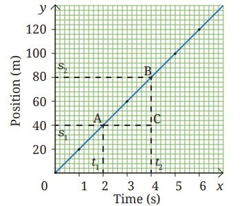
Geometrically, BC CA is called the slope of line AB connecting initial position A and final position B in Fig. 4.14. The slope of a line is the steepness of the line. The slope of a graph gives information about the rate of change of the quantity shown on y-axis with respect to the quantity shown on x-axis.
Ready to Go Beyond
Example 4.6: What does the graph shown in Fig. 4.15 indicate about the nature of motion of the vehicle?
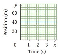
Answer: The position of the vehicle is 40 m from the origin and is not changing with time. Thus, the vehicle is at rest at 40 m from the origin. A straight line parallel to the time axis on a position-time graph represents a stationary object (In this case, the position-time graph is not the distance-time graph).
Example 4.7: The position-time graphs of two objects A and B are given in Fig. 4.16a. Which object of the magnitude of average velocity is higher?
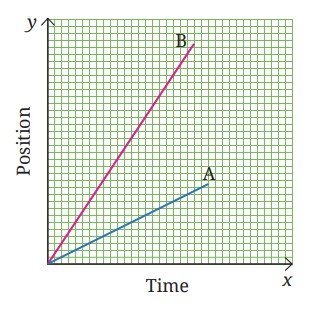
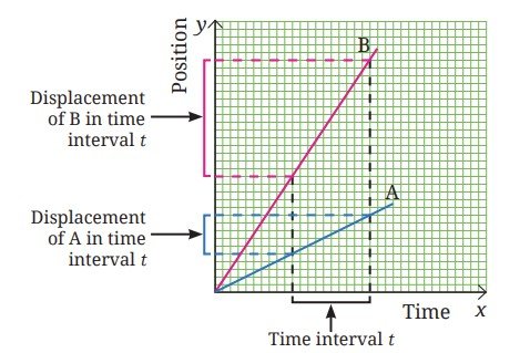
Answer: By making lines parallel to axes as shown in Fig. 4.16b, it is found that the displacement of object B is more than object A for the same time interval. That is, the slope of line for B is steeper than the slope for line A. Thus, the velocity of B is higher than that of A.
4.2.3 Velocity-time graphs
The velocity-time graph of an object in motion represents the change in its velocity with time. In a manner similar to the position-time graph, you can plot velocity-time graphs following the steps of Activity 4.3.
Let us take the example of a car moving in the same direction on a straight stretch of a highway at a steady velocity of 72 km h–1 or 20 m s–1. The velocity-time graph corresponding to it is shown in Fig. 4.17a.
Consider another car that starts moving from rest and its velocity increases with time as shown in Table 4.5. The velocity-time graph plotted for this case is shown in Fig. 4.17b.
Table 4.5: Increasing velocity
| Time | Velocity of car |
| 0 s | 0 m s–1 |
| 5 s | 2.5 m s–1 |
| 10 s | 5.0 m s–1 |
| 15 s | 7.5 m s–1 |
| 20 s | 10.0 m s–1 |
| 25 s | 12.5 m s–1 |
| 30 s | 15.0 m s–1 |
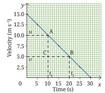
Consider yet another car moving with a velocity of 15.0 m s–1. Its velocity decreases with time as shown in Table 4.6 and its velocity-time graph is shown in Fig. 4.17c
Table 4.6: Decreasing velocity
| Time | Velocity of car |
| 0 s | 15.0 m s–1 |
| 5 s | 12.5 m s–1 |
| 10 s | 10.0 m s–1 |
| 15 s | 7.5 m s–1 |
| 20 s | 5.0 m s–1 |
| 25 s | 2.5 m s–1 |
| 30 s | 0 m s–1 |
What does the shape of the velocity-time graph indicate about the nature of motion?
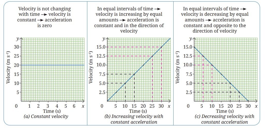
When the velocity of the car is constant, the velocity-time graph is a straight line parallel to the x-axis (Fig. 4.17a) and acceleration is zero. A straight line velocity-time graph as shown in Fig. 4.17b indicates that the velocity is increasing with a constant acceleration (in the direction of velocity). Whereas, a straight line velocity-time graph as shown in Fig. 4.17c indicates that the velocity is decreasing with a constant acceleration (opposite to the direction of velocity).
Which physical quantities can be obtained from a velocity-time graph?
Apart from finding the magnitude of velocity of the object at each instant of time, what other physical quantities can be calculated from the velocity-time graph?
Slope of the straight line on graphIn Section 4.2.2, we found that velocity can be determined from the slope of the straight line on position-time graph. What can you find from the slope of the straight line on a velocity-time graph? The slope of the line on velocity-time graph gives how fast the velocity is changing with time, i.e., the acceleration.
For the graph shown in Fig. 4.17a, there is no change in the height of the line from the x-axis, i.e., its slope is zero. Hence, the velocity is constant and the acceleration is zero in this case.
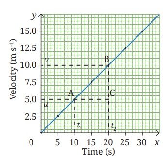
Now consider the graph shown in Fig. 4.17d which is the same as Fig. 4.17b, except for some markings. Consider a part of the line, AB. Suppose at time t1 corresponding to point A, the velocity is denoted by ‘u’, and at time t2 corresponding to point B, it is represented by ‘v’. By dividing the change in velocity (BC) by the change in time (CA), you get, a = (v-u)/(t2-t1) = BC/CA
Substituting the values from graph, we obtain the magnitude of average acceleration between the time interval from 10 s to 20 s
a = (10 ms-1 - 5 ms-1)/(20s - 10s) = 5 ms-1/10s = 0.5 ms-1
If we follow the above steps for the graph shown in Fig. 4.17e which is same as Fig. 4.17c, we obtain average acceleration to be – 0.5 m s–2. The minus sign indicates that the direction of acceleration is opposite to the direction of velocity (as the velocity is decreasing).
Can you calculate some other physical quantity from the velocity-time graph?
Area enclosed by the line on graph and time axisThe graphs shown in Fig. 4.18 are same as Fig. 4.17, except that some parts between the line on graph and the time axis are shaded. Does the area of the shaded part represent some physical quantity?
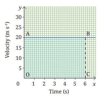
In Fig. 4.18a, OA is magnitude of the velocity and OC is the time interval.
So, area of rectangle OABC = OA × OC = velocity × time interval (Since, the velocity is constant, it is equal to the average velocity). Using Eq. (4.2a), we can say,
area of rectangle OABC = displacement
Substituting the values from graph, we obtain
displacement between 0 s and 6 s = area of OABC = 20 m s–1 × 6 s = 120 m
This is the displacement of the car from the origin in 6 seconds. You have found that the area enclosed by the velocity-time graph and the time axis for a desired time interval is equal to the displacement in that time interval.
How can you determine the displacement from the graph given in Fig. 4.18b? Suppose you want to find the displacement between 10 s to 20 s, corresponding to the graph points A and B. We calculate the area between AB and the time axis to obtain the displacement of the object which is moving with a constant acceleration. Thus,
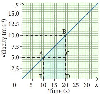
displacement between 10 s to 20 s = area of ABDE = area of the rectangle ACDE + area of the triangle ABC = (CD × DE) + (1/2 × CA × BC)
Substituting the values, we obtain
displacement = (5 m s–1 × 10 s) + (1/2 × 10 s × 5 m s–1) = 50 m + 25 m = 75 m
This is the displacement of the car between 10 s and 20 s.
We learnt that by finding the slope and area from velocity-time graph for motion with constant acceleration, we can determine acceleration and displacement, respectively.
You learnt how to represent motion by graphs. Let us now learn about the equations which describe the motion of an object.
4.3 Kinematic Equations for Motion in a Straight Line with Constant Acceleration
Let us consider the special case of motion with constant acceleration and try to derive some equations for analysing such motions. Since the acceleration is constant, acceleration at each instant will be equal to the average acceleration over any time interval.
Using the definition of average acceleration given by Eq. (4.3c),
where u is initial velocity at t = 0 s, v is final velocity at time t, time interval is t – 0 = t, over which the change in velocity occurs and a is the acceleration, we can write
This equation allows us to calculate velocity (v) at all times if initial velocity (u) and acceleration (a) are known.
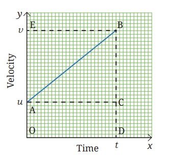
The velocity-time graph of Eq. (4.4a) is as shown in Fig. 4.19. This is similar to the graph shown in Fig. 4.18 but now the initial velocity of the object is not zero. The initial velocity (represented by AO) is u and the final velocity at time t (represented by EO) is v. The graph is a straight line indicating that the velocity changes with constant acceleration. The slope of the graph gives the acceleration.
As learnt in the earlier section, the displacement s of the object during the time interval t is given by the area enclosed within OABD. Thus,
= area of the rectangle OACD + area of the triangle ABC
= (AO × DO) + (1/2 × CA × BC)
Substituting AO = u, DO = CA = t and BC = BD – CD = EO – AO = (v – u), we obtain
Substituting the value of (v – u) from Eq. (4.4a),
s = ut + 1/2 × at 2(4.4b)
These two equations (Eq. 4.4a and Eq. 4.4b) are the primary equations. Combining these equations in different ways, we can obtain three more equations. Let us derive one of those by eliminating t in Eq. (4.4b) (the remaining two equations are given as an exercise in ‘ The Journey Beyond’ at the end of the chapter).
From Eq. (4.4a), we get
Substituting this in Eq. (4.4b), we obtain
s = u[(v-u)/a] + 1/2×a[(v-u)/a]2
⇒ s = (uv-u2)/a + (u2 + v2 - 2uv)/2a
⇒ s = (2uv - 2u2 + u2 + v2 - 2uv)/2a
⇒ s = (- u2 + v2)/2a
⇒ 2as = (- u2 + v2)
For the motion of an object in a straight line with constant acceleration, the five physical quantities-displacement (s), time interval (t), initial velocity (u), final velocity (v) and acceleration (a), can be related by the following set of equations,
These are known as kinematic equations. These equations provide a mathematical description of how the motion of an object changes with time.
Using these equations, it is possible to predict position or velocity of the object at a future time.
Note
Example 4.8: Suppose a car is moving on a highway and brakes are applied, which cause an acceleration of – 4 m s–2. How much will be the distance travelled by the car before coming to a stop, if the car was moving with a velocity of (i) 54 km h–1, and (ii) 108 km h–1 when the brakes were applied?
Answer:
Given: a = – 4 m s–2, v = 0 m s–1
Suppose the initial velocity is u and the distance travelled is s.
(i) u = 54 km h–1 = 15 m s–1
(ii) u = 108 km h–1 = 30 m s–1
Using Eq. (4.4c)
v2 = u2 + 2as
(0 ms–1)2 = u2 + 2×(-4 ms–2) × s
0 = u2-8×s
⇒ s = u2/8
Substituting the value of u, we obtain (i) 28.1 m, and (ii) 112.5 m.
Bridging Science and Society

There is a vehicle-to-vehicle (V2V) communication technology, now being developed in many countries including India, which allows vehicles to exchange signals and warns drivers of possible collisions.
Till now, in this chapter, we have been discussing about motion in a straight line which is also called motion in one dimension. Let us now explore motion in a plane.
4.4 Motion in a Plane
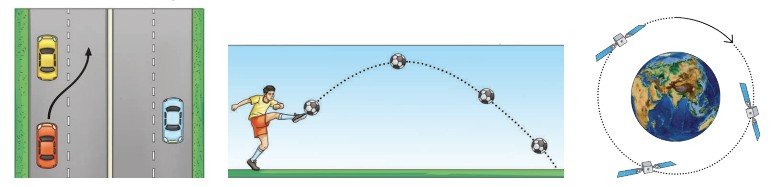
Motion in a plane, such as a vehicle overtaking another, the path of a kicked ball or a satellite moving in a circular path, is called motion in two dimensions (Fig. 4.21).
4.4.1 Uniform circular motion
Do you remember learning about circular motion in an earlier grade? When an object moves in a circular path, its motion is called circular motion.
Suppose a child is sitting on a moving merry-go-around. The child, moving on a circular path, moves from A to B to C as shown in Fig. 4.22. What is the distance travelled by the child? What is their displacement from their original position? The distance travelled by the child is the curve ABC and displacement is the straight-line AC. As you can see both are not equal.
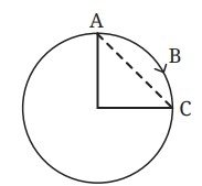
What is the distance travelled by the child in making one revolution (going round the circle once)? It is equal to the circumference of the circle. So, if the radius of the circular path is R, the distance travelled by the child in making one revolution is 2 R. On the other hand, the displacement is zero, since the child comes back to its original position after making one revolution.
If an object takes time T to make one revolution, its average speed vav will be (using Eq. 4.1)
while the average velocity during the time interval T will be 0, since the displacement is 0.
Let us now consider a particular case of circular motion where the speed of the object is constant. When an object moves in a circular path with constant (uniform) speed, its motion is called uniform circular motion.
In case of uniform circular motion, the speed is constant but what about the direction of velocity at an instant? Is it changing?
Note
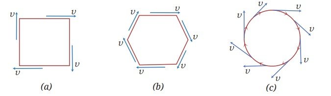
Imagine an athlete running along a closed path. In Fig. 4.23a, the athlete follows a rectangular track (ABCD), running at a uniform speed on the straight sections (AB, BC, CD and DA). The athlete changes direction four times to complete one round. In Fig. 4.23b, the athlete is running along a hexagonal path. In this case, the athlete changes direction six times to complete one round. What happens if we keep increasing the number of sides indefinitely? As the number of sides increases, the athlete has to take turns more and more frequently. Finally, the track approaches a circle, with each side decreasing to a point and the direction of athlete’s velocity changes continuously
Note
Activity 4.5: Let us investigate
- Take a ring, such as an adhesive tape ring and one marble.
- Place the ring flat on a smooth surface and throw the marble inside the ring in a way that it rotates along the inner boundary of the ring (Fig. 4.24).
![Image]()
Fig. 4.24: A marble moving inside a ring - Predict what will happen if you lift the ring while the marble is moving.
- Now, after one or two complete revolutions of the marble, pick up the ring without disturbing the motion of the marble. What do you observe? Does the marble continue moving in a circular motion? Or does it move in some other manner?
- Repeat the activity multiple times to confirm the result.
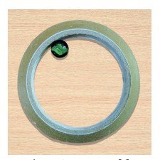
When the marble is released by lifting the ring, it moves in a straight line. This happened because once the marble is released, it continues to move in the direction it has been moving at the instant the ring was removed. You will learn the reason for this in a later chapter.
Ready to Go Beyond
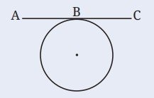
Note
You know that acceleration is non-zero if the velocity of an object changes. The velocity changes if either its magnitude or direction, or both changes. In uniform circular motion, the motion of the object is accelerated because the direction of its velocity continuously changes.
Ready to Go Beyond
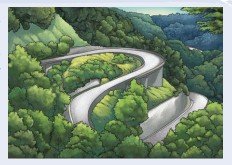
In real world, the conditions for uniform circular motion — constant speed and a circular path — are often not met. So, uniform circular motion is an idealised model of the real-world situations. Still, it is a useful model as it serves as the foundation for more complex real-world situations, such as motion of planets revolving around the Sun or a vehicle making a circular turn.
At a Glance
- The distance and direction of an object with respect to the reference point, at any instant of time, describes the position of the object at that instant of time.
- If the position of the object with respect to a reference point changes with time, the object is said to be in motion.
- Displacement is the net change in the position of the object between two given instants of time.
- The average speed of an object is the total distance travelled divided by the time interval during which this distance is covered.
- The average velocity of an object in a time interval is the change in position (also known as displacement) divided by the time interval in which the change in position (or displacement) occurs.
- The average acceleration of an object over a time interval is the change in its velocity divided by the time interval.
- For the motion of an object in a straight line with constant acceleration, the five physical quantities — displacement (s), time interval (t), initial velocity (u), final velocity (v) and acceleration (a), can be related by the following set of kinematic equations,
v = u + at
s = ut + 1/2at 2
v2 = u2 + 2as - When an object moves in a circular path with constant (uniform) speed, its motion is called the uniform circular motion.
Revise, Reflect, Refine
- My father went to a shop from home which is located at a distance of 250 m on a straight road. On reaching there, he discovered that he forgot to carry a cloth bag. He came home to take it, went to the shop again, bought provisions and came back home. How much was the total distance travelled by him? What was his displacement from home?
- A student runs from the ground floor to the fourth floor of a school building to collect a book and then comes down to their classroom on the second floor. If the height of each floor is 3 m, find:
- the total vertical distance travelled, and
- their displacement from the starting point.
- A girl is riding her scooter and finds that its speedometer reading is constant. Is it possible for her scooter to be accelerating and if so, how?
- A car starts from rest and its velocity reaches 24ms–1 in 6 s. Find the average acceleration and the distance travelled in these 6 s.
- A motorbike moving with initial velocity 28 ms–1 and constant acceleration stops after travelling 98 m. Find the acceleration of the motorbike and the time taken to come to a stop.
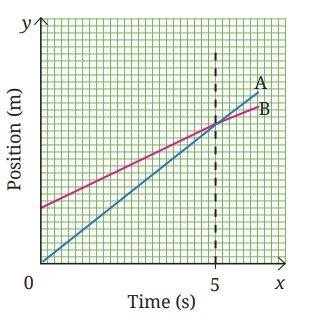
- Fig. 4.27 shows a position-time graph of two objects A and B that are moving along the parallel tracks in the same direction. Do objects A and B ever have equal velocity? Justify your answer.
![Image]()
Fig. 4.27
![Image]()
Fig. 4.28
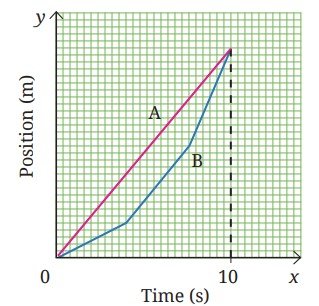
- A graph in Fig. 4.28 shows the change in position with time for two objects A and B moving in a straight line from 0 to 10 seconds. Choose the correct option(s).
- The average velocity of both over the 10 s time interval is equal since they have the same initial and final positions.
- The average speeds of both over the 10 s time interval are equal since both cover equal distance in equal time.
- The average speed of A over the 10 s time interval is lower than that of B since it covers a shorter distance than B in 10 seconds.
- The average speed of A over the 10 s time interval is greater than that of B since B’s speed is lower than A’s in some segments.
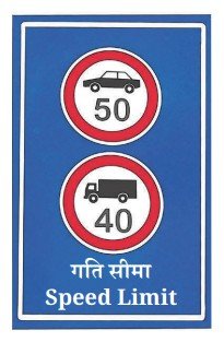
- A truck driver driving at the speed of 54 km h–1 notices a road sign with a speed limit of 40 km h–1 (Fig. 4.29) for trucks. He slows down to 36 km h–1 in 36 s. What was the distance travelled by him during this time? Assume the acceleration to be constant while slowing down.
![Image]()
Fig. 4.29 - A car starts from rest and accelerates uniformly to 20ms–1 in 5 seconds. It then travels at 20ms–1 for 10 seconds and finally applies the brake (with uniform acceleration) to stop in 6 seconds. Find the total distance travelled.
- A bus is travelling at 36kmh–1 when the driver sees an obstacle 30 m ahead. The driver takes 0.5 seconds to react before pressing the brake. Once the brake is applied, the velocity of the bus reduces with constant acceleration of 2.5 ms–2. Will the bus be able to stop before reaching the obstacle?
- A student said, “The Earth moves around the Sun”. In this context, discuss whether an object kept on the Earth can be considered to be at rest.
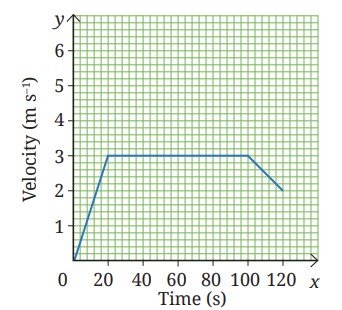
- The velocity-time graph from 0 s to 120 s for a cyclist is shown in Fig. 4.30. Shade the areas (in different colours) representing the displacement of the cyclist
- while cyclist is moving with constant velocity
- when the velocity of cyclist is decreasing.
![Image]()
Fig. 4.30
![Image]()
Fig. 4.31
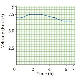
- A girl is preparing for her first marathon by running on a straight road. She uses a smartwatch to calculate her running speed at different intervals. The graph (Fig. 4.31) depicts her velocity versus time. Estimate the running distance based on the graph.
- On entering a state highway, a car continues to move with a constant velocity of 6 ms–1 for 2 minutes and then accelerates with a constant acceleration 1 ms–2 for 6 seconds. Find the displacement of the car on the state highway in the 2 min 6 s time interval by drawing a velocity-time graph for its motion.
- Two cars A and B start moving with a constant acceleration from rest in a straight line. Car A attains a velocity of 5 ms–1 in 5 s. Car B attains a velocity of 3 ms–1 in 10 s. Plot the velocity-time graphs for both the cars in the same graph. Using the graph, calculate the displacement mentioned in the two time intervals (Hint: Calculate the acceleration in both cases. Then calculate their velocities at five instants of time to plot the graph).
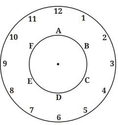
- Rohan studies science from 6 PM to 7:30 PM at home. Consider the tip of the minute’s hand of the wall clock. During the given time interval, what is its:
- distance travelled,
- displacement,
- speed, and
- velocity.
![Image]()
Fig. 4.32

The Journey Beyond
- Take a cardboard disc (radius ~ 8 cm) (Fig. 4.33). Write numbers 1 to 12 on the outer part (7 cm from the centre) and the letters ‘ABCDEF’ on the inner part (4 cm from the centre), using the same font size. Spin the disc slowly, then faster and observe how the numbers and letters appear. Why do the numbers fade or disappear while the letters remain visible? Are the speeds of the numbers and letters the same or different? Justify your answer.
![Image]()
Fig. 4.33 - Many smartphones have an inbuilt accelerometer that can detect very small accelerations. Install an app, such as Phyphox (phyphox.org) and open ‘Accelerometer’ (without g). Note the readings when (i) the phone is on an outstretched palm, and (ii) the phone is kept on the floor. What differences do you observe? What does this tell you about motion and acceleration in real situations? (Such tiny, involuntary movements are also studied in medical research, for example, in movement disorders) This activity is recommended to be performed as a classroom group activity facilitated by teacher
- For motion in a straight line with constant acceleration, we derived two primary equations given by Eq. (4.4a) and (4.4b). Using these two equations, three more equations can be derived, out of which we derived one given in Eq. (4.4c). Derive the remaining two equations given below
s = vt - 1/2at 2 In mathematics, you have learnt the formula for calculating the area of a trapezium. Using that formula, derive the second equation given above.
s = 1/2(u + v)t - Plot graphs for data given in Table 4.4, using different X and Y scales, on different graph papers. Compare the graphs to find how the appearance of graph is affected by the choice of scales and decide which scale is better and why. Now repeat this with any graph plotting app. Such apps generally automatically adjust the axes to fit the data well on the screen.
- Talk to a motor mechanic about how a vehicle’s braking or stopping distance is affected by: (i) wet roads, (ii) worn-out tyres, (iii) higher vehicle mass, (iv) driving at night, (v) fog, (vi) severe weather (rain, snow, storm), and (vii) driver reaction time. Using this information, design safety posters for your school and prepare a short skit to present it in the assembly.