Table of Contents

Unit 5
STATES OF MATTER

After studying this unit you will be able to
• explain the existence of different states of matter in terms of balance between intermolecular forces and thermal energy of particles;
• explain the laws governing behaviour of ideal gases;
• apply gas laws in various real life situations;
• explain the behaviour of real gases;
• describe the conditions required for liquifaction of gases;
• realise that there is continuity in gaseous and liquid state;
• differentiate between gaseous state and vapours; and
• explain properties of liquids in terms of intermolecular attractions.
The snowflake falls, yet lays not long
Its feath’ry grasp on Mother Earth
Ere Sun returns it to the vapors Whence it came,
Or to waters tumbling down the rocky slope.
Rod O’ Connor
Introduction
In previous units we have learnt about the properties related to single particle of matter, such as atomic size, ionization enthalpy, electronic charge density, molecular shape and polarity, etc. Most of the observable characteristics of chemical systems with which we are familiar represent bulk properties of matter, i.e., the properties associated with a collection of a large number of atoms, ions or molecules. For example, an individual molecule of a liquid does not boil but the bulk boils. Collection of water molecules have wetting properties; individual molecules do not wet. Water can exist as ice, which is a solid; it can exist as liquid; or it can exist in the gaseous state as water vapour or steam. Physical properties of ice, water and steam are very different. In all the three states of water chemical composition of water remains the same i.e., H2O. Characteristics of the three states of water depend on the energies of molecules and on the manner in which water molecules aggregate. Same is true for other substances also.
Chemical properties of a substance do not change with the change of its physical state; but rate of chemical reactions do depend upon the physical state. Many times in calculations while dealing with data of experiments we require knowledge of the state of matter. Therefore, it becomes necessary for a chemist to know the physical laws which govern the behaviour of matter in different states. In this unit, we will learn more about these three physical states of matter particularly liquid and gaseous states. To begin with, it is necessary to understand the nature of intermolecular forces, molecular interactions and effect of thermal energy on the motion of particles because a balance between these determines the state of a substance.
5.1 Intermolecular Forces
Intermolecular forces are the forces of attraction and repulsion between interacting particles (atoms and molecules). This term does not include the electrostatic forces that exist between the two oppositely charged ions and the forces that hold atoms of a molecule together i.e., covalent bonds.
Attractive intermolecular forces are known as van der Waals forces, in honour of Dutch scientist Johannes van der Waals (1837-1923), who explained the deviation of real gases from the ideal behaviour through these forces. We will learn about this later in this unit. van der Waals forces vary considerably in magnitude and include dispersion forces or London forces, dipole-dipole forces, and dipole-induced dipole forces. A particularly strong type of dipole-dipole interaction is hydrogen bonding. Only a few elements can participate in hydrogen bond formation, therefore it is treated as a separate category. We have already learnt about this interaction in Unit 4.
At this point, it is important to note that attractive forces between an ion and a dipole are known as ion-dipole forces and these are not van der Waals forces. We will now learn about different types of van der Waals forces.
5.1.1 Dispersion Forces or London Forces
Atoms and nonpolar molecules are electrically symmetrical and have no dipole moment because their electronic charge cloud is symmetrically distributed. But a dipole may develop momentarily even in such atoms and molecules. This can be understood as follows. Suppose we have two atoms ‘A’ and ‘B’ in the close vicinity of each other (Fig. 5.1a). It may so happen that momentarily electronic charge distribution in one of the atoms, say ‘A’, becomes unsymmetrical i.e., the charge cloud is more on one side than the other (Fig. 5.1 b and c). This results in the development of instantaneous dipole on the atom ‘A’ for a very short time. This instantaneous or transient dipole distorts the electron density of the
other atom ‘B’, which is close to it and as a consequence a dipole is induced in the atom ‘B’.
The temporary dipoles of atom ‘A’ and ‘B’ attract each other. Similarly temporary dipoles are induced in molecules also. This force of attraction was first proposed by the German physicist Fritz London, and for this reason force of attraction between two temporary dipoles is known as London force. Another name for this force is dispersion force. These forces are always attractive and interaction energy is inversely proportional to the sixth power of the distance between two interacting particles (i.e., 1/r6 where r is the distance between two particles). These forces are important only at short distances (~500 pm) and their magnitude depends on the polarisability of the particle.
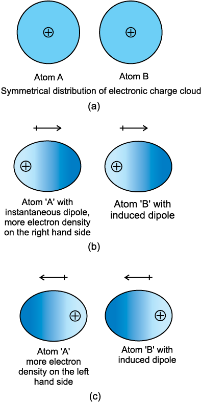
Fig. 5.1 Dispersion forces or London forces between atoms.
5.1.2 Dipole - Dipole Forces
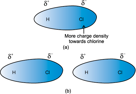
Dipole-dipole forces act between the molecules possessing permanent dipole. Ends of the dipoles possess “partial charges” and these charges are shown by Greek letter delta (δ). Partial charges are always less than the unit electronic charge (1.6×10⁻¹⁹ C). The polar molecules interact with neighbouring molecules. Fig 5.2 (a) shows electron cloud distribution in the dipole of hydrogen chloride and Fig. 5.2 (b) shows dipole-dipole interaction between two HCl molecules. This interaction is stronger than the London forces but is weaker than ion-ion interaction because only partial charges are involved. The attractive force decreases with the increase of distance between the dipoles. As in the above case here also, the interaction energy is inversely proportional to distance between polar molecules. Dipole-dipole interaction energy between stationary polar molecules (as in solids) is proportional to 1/r3 and that between rotating polar molecules is proportional to 1/r 6, where r is the distance between polar molecules. Besides dipole-dipole interaction, polar molecules can interact by London forces also. Thus cumulative effect is that the total of intermolecular forces in polar molecules increase.
5.1.3 Dipole–Induced Dipole Forces
This type of attractive forces operate between the polar molecules having permanent dipole and the molecules lacking permanent dipole. Permanent dipole of the polar molecule induces dipole on the electrically neutral molecule by deforming its electronic cloud (Fig. 5.3). Thus an induced dipole is developed in the other molecule. In this case also interaction energy is proportional to 1/r6 where r is the distance between two molecules. Induced dipole moment depends upon the dipole moment present in the permanent dipole and the polarisability of the electrically neutral molecule. We have already learnt in Unit 4 that molecules of larger size can be easily polarized. High polarisability increases the strength of attractive interactions.
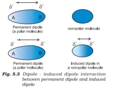
In this case also cumulative effect of dispersion forces and dipole-induced dipole interactions exists.
5.1.4 Hydrogen bond
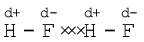
As already mentioned in section (5.1); this is special case of dipole-dipole interaction. We have already learnt about this in Unit 4. This is found in the molecules in which highly polar N–H, O–H or H–F bonds are present. Although hydrogen bonding is regarded as being limited to N, O and F; but species such as  may also participate in hydrogen bonding. Energy of hydrogen bond varies between 10 to 100 kJ mol–1. This is quite a significant amount of energy; therefore, hydrogen bonds are powerful force in determining the structure and properties of many compounds, for example proteins and nucleic acids. Strength of the hydrogen bond is determined by the coulombic interaction between the lone-pair electrons of the electronegative atom of one molecule and the hydrogen atom of other molecule. Following diagram shows the formation of hydrogen bond.
Intermolecular forces discussed so far are all attractive. Molecules also exert repulsive forces on one another. When two molecules are brought into close contact with each other, the repulsion between the electron clouds and that between the nuclei of two molecules comes into play. Magnitude of the repulsion rises very rapidly as the distance separating the molecules decreases. This is the reason that liquids and solids are hard to compress. In these states molecules are already in close contact; therefore they resist further compression; as that would result in the increase of repulsive interactions.
5.2 Thermal Energy
Thermal energy is the energy of a body arising from motion of its atoms or molecules. It is directly proportional to the temperature of the substance. It is the measure of average
kinetic energy of the particles of the matter and is thus responsible for movement of particles. This movement of particles is called thermal motion.
5.3 Intermolecular Forces vs Thermal Interactions
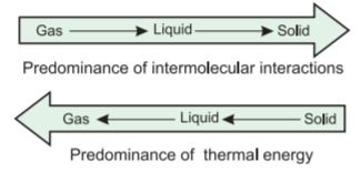
We have already learnt that intermolecular forces tend to keep the molecules together but thermal energy of the molecules tends to keep them apart. Three states of matter are the result of balance between intermolecular forces and the thermal energy of the molecules.
When molecular interactions are very weak, molecules do not cling together to make liquid or solid unless thermal energy is reduced by lowering the temperature. Gases do not liquify on compression only, although molecules come very close to each other and intermolecular forces operate to the maximum. However, when thermal energy of molecules is reduced by lowering the temperature; the gases can be very easily liquified. Predominance of thermal energy and the molecular interaction energy of a substance in three states is depicted as follows :
We have already learnt the cause for the existence of the three states of matter. Now we will learn more about gaseous and liquid states and the laws which govern the behaviour of matter in these states. We shall deal with the solid state in class XII.
5.4 The Gaseous State
This is the simplest state of matter. Throughout our life we remain immersed in the ocean of air which is a mixture of gases. We spend our life in the lowermost layer of the atmosphere called troposphere, which is held to the surface of the earth by gravitational force. The thin layer of atmosphere is vital to our life. It shields us from harmful radiations and contains substances like dioxygen, dinitrogen, carbon dioxide, water vapour, etc.
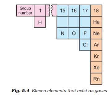
Let us now focus our attention on the behaviour of substances which exist in the gaseous state under normal conditions of temperature and pressure. A look at the periodic table shows that only eleven elements exist as gases under normal conditions (Fig 5.4).
The gaseous state is characterized by the following physical properties.
• Gases are highly compressible.
• Gases exert pressure equally in all directions.
• Gases have much lower density than the solids and liquids.
• The volume and the shape of gases are not fixed. These assume volume and shape of the container.
• Gases mix evenly and completely in all proportions without any mechanical aid.
Simplicity of gases is due to the fact that the forces of interaction between their molecules are negligible. Their behaviour is governed by same general laws, which were discovered as a result of their experimental studies. These laws are relationships between measurable properties of gases. Some of these properties like pressure, volume, temperature and mass are very important because relationships between these variables describe state of the gas. Interdependence of these variables leads to the formulation of gas laws. In the next section we will learn about gas laws.
5.5 The Gas Laws
The gas laws which we will study now are the result of research carried on for several centuries on the physical properties of gases. The first reliable measurement on properties of gases was made by Anglo-Irish scientist Robert Boyle in 1662. The law which he formulated is known as Boyle’s Law. Later on attempts to fly in air with the help of hot air balloons motivated Jaccques Charles and Joseph Lewis Gay Lussac to discover additional gas laws. Contribution from Avogadro and others provided lot of information about gaseous state.
5.5.1 Boyle’s Law (Pressure - Volume Relationship)
On the basis of his experiments, Robert Boyle reached to the conclusion that at constant temperature, the pressure of a fixed amount (i.e., number of moles n) of gas varies inversely with its volume. This is known as Boyle’s law. Mathematically, it can be written as
 ( at constant T and n) (5.1)
 (5.2)
(5.2)
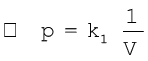
where k1 is the proportionality constant. The value of constant k1 depends upon the amount of the gas, temperature of the gas and the units in which p and V are expressed.
On rearranging equation (5.2) we obtain
pV = k1 (5.3)
It means that at constant temperature, product of pressure and volume of a fixed amount of gas is constant.
If a fixed amount of gas at constant temperature T occupying volume V1 at pressure p1 undergoes expansion, so that volume becomes V2 and pressure becomes p2, then according to Boyle’s law :
p1V1 = p2V2= constant (5.4)
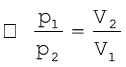 (5.5)
(5.5)
Figure 5.5 shows two conventional ways of graphically presenting Boyle’s law.
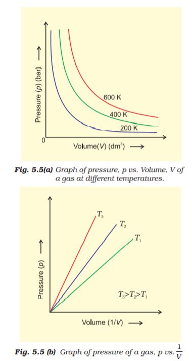
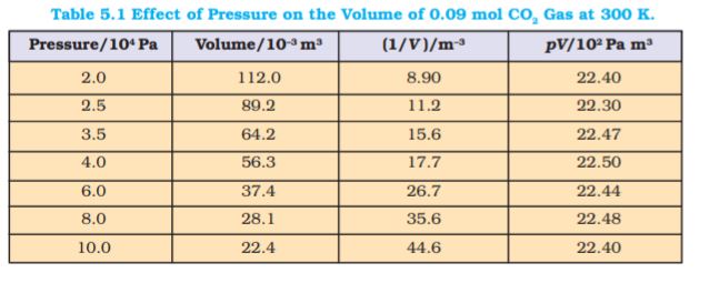
Fig. 5.5 (a) is the graph of equation (5.3) at different temperatures. The value of k1 for each curve is different because for a given mass of gas, it varies only with temperature. Each curve corresponds to a different constant temperature and is known as an isotherm (constant temperature plot). Higher curves correspond to higher temperature. It should be noted that volume of the gas doubles if pressure is halved. Table 5.1 gives effect of pressure on volume of 0.09 mol of CO2 at
300 K.
Fig 5.5 (b) represents the graph between p and  . It is a straight line passing through origin. However at high pressures, gases deviate from Boyle’s law and under such conditions a straight line is not obtained in the graph.
Experiments of Boyle, in a quantitative manner prove that gases are highly compressible because when a given mass of a gas is compressed, the same number of molecules occupy a smaller space. This means that gases become denser at high pressure. A relationship can be obtained between density and pressure of a gas by using Boyle’s law:
By definition, density ‘d’ is related to the mass ‘m’ and the volume ‘V’ by the relation  . If we put value of V in this equation from Boyle’s law equation, we obtain the relationship.
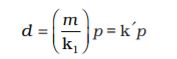
This shows that at a constant temperature, pressure is directly proportional to the density of a fixed mass of the gas.
Problem 5.1
A balloon is filled with hydrogen at room temperature. It will burst if pressure exceeds 0.2 bar. If at 1 bar
pressurethe gas occupies 2.27 L volume, upto what volume can the balloon be expanded ?
Solution
According to Boyle’s Law p1V1 = p2V2
If p1 is 1 bar, V1 will be 2.27 L
If p2 = 0.2 bar, then 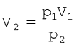
 =11.35 L
Since balloon bursts at 0.2 bar pressure, the volume of balloon should be less than 11.35 L.
5.5.2 Charles’ Law (Temperature - Volume Relationship)
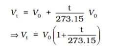
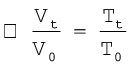
Charles and Gay Lussac performed several experiments on gases independently to improve upon hot air balloon technology. Their investigations showed that for a fixed mass of a gas at constant pressure, volume of a gas increases on increasing temperature and decreases on cooling. They found that for each degree rise in temperature, volume of a gas increases by  of the original volume of the gas at 0 °C. Thus if volumes of the gas at 0 °C and at t °C are V0 and Vt respectively, then
At this stage, we define a new scale of temperature such that t °C on new scale is given by T = 273.15 + t and 0 °C will be given by T0 = 273.15. This new temperature scale is called the Kelvin temperature scale or Absolute temperature scale.
Thus 0°C on the celsius scale is equal to 273.15 K at the absolute scale. Note that degree sign is not used while writing the temperature in absolute temperature scale, i.e., Kelvin scale. Kelvin scale of temperature is also called Thermodynamic scale of temperature and is used in all scientific works.
Thus we add 273 (more precisely 273.15) to the celsius temperature to obtain temperature at Kelvin scale.
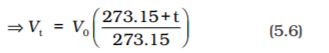
If we write Tt = 273.15 + t and T0 = 273.15
in the equation (5.6) we obtain the relationship
 (5.7)
(5.7)
Thus we can write a general equation as follows.
 (5.8)
(5.8)
 (5.9)
(5.9)
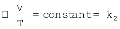
Thus V = k2 T (5.10)
The value of constant k2 is determined by the pressure of the gas, its amount and the units in which volume V is expressed.
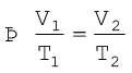
Equation (5.10) is the mathematical expression for Charles’ law, which states that pressure remaining constant, the volume of a fixed mass of a gas is directly proportional to its absolute temperature. Charles found that for all gases, at any given pressure, graph of volume vs temperature (in celsius) is a straight line and on extending to zero volume, each line intercepts the temperature axis at – 273.15 °C. Slopes of lines obtained at different pressure are different but at zero volume all the lines meet the temperature axis at – 273.15 °C (Fig. 5.6).
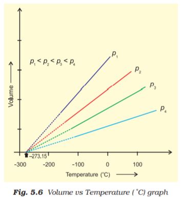
Each line of the volume vs temperature graph is called isobar.
Observations of Charles can be interpreted if we put the value of t in equation (5.6) as
– 273.15 °C. We can see that the volume of the gas at – 273.15 °C will be zero. This means that gas will not exist. In fact all the gases get liquified before this temperature is reached. The lowest hypothetical or imaginary temperature at which gases are supposed to occupy zero volume is called Absolute zero.
All gases obey Charles’ law at very low pressures and high temperatures.
Problem 5.2
On a ship sailing in Pacific Ocean where temperature is 23.4°C, a balloon is filled with 2 L air. What will be the
volume of the balloon when the ship reaches Indian ocean, where temperature is 26.1°C ?
Solution
V1 = 2 L T2 = 26.1 + 273
T1 = (23.4 + 273) K = 299.1 K
= 296.4 K
From Charles law
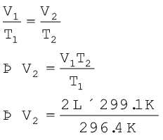
= 2L × 1.009
= 2.018L
5.5.3 Gay Lussac’s Law (Pressure- Temperature Relationship)
Pressure in well inflated tyres of automobiles is almost constant, but on a hot summer day this increases considerably and tyre may burst if pressure is not adjusted properly. During winters, on a cold morning one may find the pressure in the tyres of a vehicle decreased considerably. The mathematical relationship between pressure and temperature was given by Joseph Gay Lussac and is known as Gay Lussac’s law. It states that at constant volume, pressure of a fixed amount of a gas varies directly with the temperature . Mathematically,
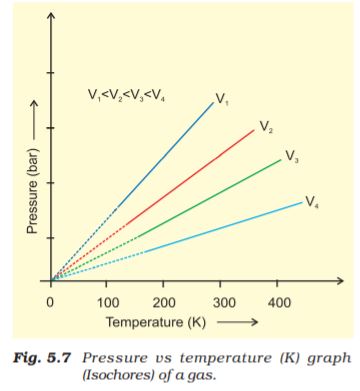
This relationship can be derived from Boyle’s law and Charles’ Law. Pressure vs temperature (Kelvin) graph at constant molar volume is shown in Fig. 5.7. Each line of this graph is called isochore.
5.5.4 Avogadro Law (Volume - Amount Relationship)
In 1811 Italian scientist Amedeo Avogadro tried to combine conclusions of Dalton’s atomic theory and Gay Lussac’s law of combining volumes (Unit 1) which is now known as Avogadro law. It states that equal volumes of all gases under the same conditions of temperature and pressure contain equal number of molecules. This means that as long as the temperature and pressure remain constant, the volume depends upon number of molecules of the gas or in other words amount of the gas. Mathematically we can write
 where n is the number of moles of the gas.
 (5.11)
The number of molecules in one mole of a gas has been determined to be 6.022 ×10²³ and is known as Avogadro constant. You
will find that this is the same number which we came across while discussing definition of a ‘mole’ (Unit 1).
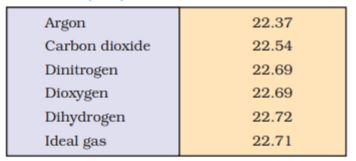
Since volume of a gas is directly proportional to the number of moles; one mole of each gas at standard temperature and pressure (STP)* will have same volume. Standard temperature and pressure means 273.15 K (0°C) temperature and 1 bar (i.e., exactly 105 pascal) pressure. These
values approximate freezing temperature of water and atmospheric pressure at sea level. At STP molar volume of an ideal gas or a combination of ideal gases is 22.71098 L mol–1.
Molar volume of some gases is given in (Table 5.2).
Number of moles of a gas can be calculated as follows
n =  (5.12)
Where m = mass of the gas under investigation and M = molar mass
Thus,
V = k4 (5.13)
Equation (5.13) can be rearranged as follows :
M = k4  = k4d (5.14)
Here ‘d’ is the density of the gas. We can conclude from equation (5.14) that the density of a gas is directly proportional to its molar mass.
A gas that follows Boyle’s law, Charles’ law and Avogadro law strictly is called an ideal gas. Such a gas is hypothetical. It is assumed that intermolecular forces are not present between the molecules of an ideal gas. Real gases follow these laws only under certain specific conditions when forces of interaction are practically negligible. In all other situations these deviate from ideal behaviour. You will learn about the deviations later in this unit.
5.6 Ideal Gas Equation
The three laws which we have learnt till now can be combined together in a single equation which is known as ideal gas equation.
At constant T and n; V 2029.png Boyle’s Law
At constant p and n; V 2041.png T Charles’ Law
At constant p and T ; V 2054.png n Avogadro LawThus,
 (5.15)
 (5.16)
where R is proportionality constant. On rearranging the equation (5.16) we obtain
pV = n RT (5.17)
 (5.18)
R is called gas constant. It is same for all gases. Therefore it is also called Universal Gas Constant. Equation (5.17) is called ideal gas equation.
Equation (5.18) shows that the value of R depends upon units in which p, V and T are measured. If three variables in this equation are known, fourth can be calculated. From this equation we can see that at constant temperature and pressure n moles of any gas will have the same volume because 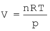 and n,R,T and p are constant. This equation will be applicable to any gas, under those conditions when behaviour of the gas approaches ideal behaviour. Volume of one mole of an ideal gas under STP conditions (273.15 K and 1 bar pressure) is 22.710981 L mol–1. Value
of R for one mole of an ideal gas can be calculated under these conditions
as follows :
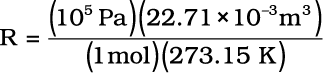
= 8.314 Pa m3 K–1 mol–1
= 8.314 × 10⁻² bar L K–1 mol–1
= 8.314 J K–1 mol–1
At STP conditions used earlier (0 °C and 1 atm pressure), value of R is 8.20578 × 10⁻² L atm K–1 mol–1.
Ideal gas equation is a relation between four variables and it describes the state of any gas, therefore, it is also called equation of state.
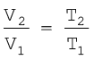
Let us now go back to the ideal gas equation. This is the relationship for the simultaneous variation of the variables. If temperature, volume and pressure of a fixed amount of gas vary from T1, V1 and p1 to T2, V2 and p2 then we can write
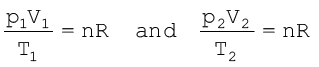
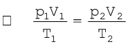 (5.19)
The previous standard is still often used, and applies to all chemistry data more than decade old. In this definition STP denotes the same temperature of 0°C (273.15 K), but a slightly higher pressure of 1 atm (101.325 kPa). One mole of any gas of a combination of gases occupies 22.413996 L of volume at STP.
Standard ambient temperature and pressure (SATP), conditions are also used in some scientific works. SATP conditions means 298.15 K and 1 bar (i.e., exactly 105 Pa). At SATP (1 bar and 298.15 K), the molar volume of an ideal gas is 24.789 L mol–1.
Equation (5.19) is a very useful equation. If out of six, values of five variables are known, the value of unknown variable can be calculated from the equation (5.19). This equation is also known as Combined gas law.
Problem 5.3
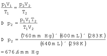
At 25°C and 760 mm of Hg pressure a gas occupies 600 mL volume. What will be its pressure at a height
wheretemperature is 10°C and volume of the gas is 640 mL.
Solution
p1 = 760 mm Hg, V1= 600 mL
T1 = 25 + 273 = 298 K
V2 = 640 mL and T2 = 10 + 273 = 283 K
According to Combined gas law
5.6.1 Density and Molar Mass of a Gaseous Substance
Ideal gas equation can be rearranged as follows:

Replacing n by  , we get
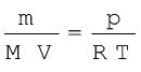 (5.20)
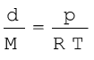 (where d is the density) (5.21)
On rearranging equation (5.21) we get the relationship for calculating molar mass of a gas.
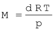 (5.22)
5.6.2 Dalton’s Law of Partial Pressures
The law was formulated by John Dalton in 1801. It states that the total pressure exerted by the mixture of non-reactive gases is equal to the sum of the partial pressures of individual gases i.e., the pressures which these gases would exert if they were enclosed separately in the same volume and under the same conditions of temperature. In a mixture of gases, the pressure exerted by the individual gas is called partial pressure. Mathematically,
pTotal = p1+p2+p3+......(at constant T, V) (5.23)
where pTotal is the total pressure exerted by the mixture of gases and p1, p2 , p3 etc. are partial pressures of gases.
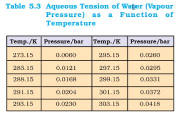
Gases are generally collected over water and therefore are moist. Pressure of dry gas can be calculated by subtracting vapour pressure of water from the total pressure of the moist gas which contains water vapours also. Pressure exerted by saturated water vapour is called aqueous tension. Aqueous tension of water at different temperatures is given in Table 5.3.
pDry gas = pTotal – Aqueous tension (5.24)
Partial pressure in terms of mole fraction
Suppose at the temperature T, three gases, enclosed in the volume V, exert partial pressure p1, p2 and p3 respectively, then,
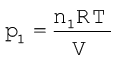 (5.25)
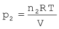 (5.26)
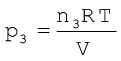 (5.27)
where n1 n2 and n3 are number of moles of these gases. Thus, expression for total pressure will be
pTotal = p1 + p2 + p3
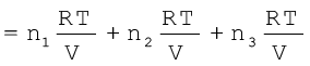
= (n1 + n2 + n3)  (5.28)
On dividing p1 by ptotal we get
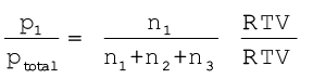
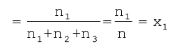
where n = n1+n2+n3
x1 is called mole fraction of first gas.
Thus, p1 = x1 ptotal
Similarly for other two gases we can write
p2 = x2 ptotal and p3 = x3 ptotal
Thus a general equation can be written as
pi = xi ptotal (5.29)
where pi and xi are partial pressure and mole fraction of ith gas respectively. If total pressure of a mixture of gases is known, the equation (5.29) can be used to find out pressure exerted by individual gases.
Problem 5.4
A neon-dioxygen mixture contains 70.6 g dioxygen and 167.5 g neon. If pressure of the mixture of gases in thecylinder
is 25 bar. What is the partial pressure of dioxygen and neon in the mixture ?
Number of moles of dioxygen 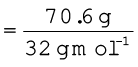
= 2.21 mol
Number of moles of neon
= 8.375 mol
Mole fraction of dioxygen 
Mole fraction of neon 
= 0.79
Alternatively,
mole fraction of neon = 1– 0.21 = 0.79
Partial pressure = mole fraction ×
of a gas total pressure
⇒ Partial pressure = 0.21 × (25 bar)
of oxygen = 5.25 bar
Partial pressure = 0.79 × (25 bar)
of neon = 19.75 bar
5.7 Kinetic Energy and Molecular Speeds
Molecules of gases remain in continuous motion. While moving they collide with each other and with the walls of the container. This results in change of their speed and redistribution of energy. So the speed and energy of all the molecules of the gas at any instant are not the same. Thus, we can obtain only average value of speed of molecules. If there are n number of molecules in a sample and their individual speeds are u1, u2, …….un, then average speed of molecules uav can be calculated as follows:
Maxwell and Boltzmann have shown that actual distribution of molecular speeds depends on temperature and molecular mass of a gas. Maxwell derived a formula for calculating the number of molecules possessing a particular speed. Fig. 5.8 shows schematic plot of number of molecules vs. molecular speed at two different temperatures T1 and T2 (T2 is higher than T1). The distribution of speeds shown in the plot is called Maxwell-Boltzmann distribution of speeds.
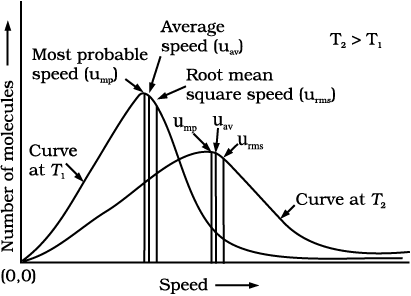
Fig. 5.8: Maxwell-Boltzmann distribution of speeds
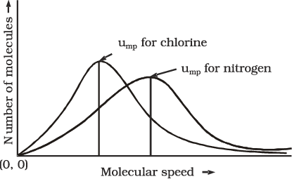
The graph shows that number of molecules possessing very high and very low speed is very small. The maximum in the curve represents speed possessed by maximum number of molecules. This speed is called most probable speed, ump. This is very close to the average speed of the molecules. On increasing the temperature most probable speed increases. Also, speed distribution curve broadens at higher temperature. Broadening of the curve shows that number of molecules moving at higher speed increases. Speed distribution also depends upon mass of molecules. At the same temperature, gas molecules with heavier mass have slower speed than lighter gas molecules. For example, at the same temperature lighter nitrogen molecules move faster than heavier chlorine molecules. Hence, at any given temperature, nitrogen molecules have higher value of most probable speed than the chlorine molecules. Look at the molecular speed distribution curve of chlorine and nitrogen given in Fig. 5.9. Though at a particular temperature the individual speed of molecules keeps changing, the distribution of speeds remains same.
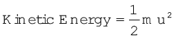
We know that kinetic energy of a particle is given by the expression:
Therefore, if we want to know average translational kinetic energy,  , for the movement of a gas particle in a straight line, we require the value of mean of square of speeds,
  , of all molecules. This is represented as follows:
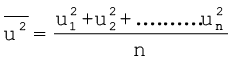
The mean square speed is the direct measure of the average kinetic energy of gas molecules. If we take the square root of the mean of the square of speeds then we get a value of speed which is different from most probable speed and average speed. This speed is called root mean square speed and is given by the expression as follows:
urms
Root mean square speed, average speed and the most probable speed have following relationship:
urms > uav > ump
The ratio between the three speeds is given below :
ump: uav : urms : : 1 : 1.128 : 1.224
5.8 Kinetic Molecular Theory of Gases
So far we have learnt the laws (e.g., Boyle’s law, Charles’ law etc.) which are concise statements of experimental facts observed in the laboratory by the scientists. Conducting careful experiments is an important aspect of scientific method and it tells us how the particular system is behaving under different conditions. However, once the experimental facts are established, a scientist is curious to know why the system is behaving in that way. For example, gas laws help us to predict that pressure increases when we compress gases but we would like to know what happens at molecular level when a gas is compressed ? A theory is constructed to answer such questions. A theory is a model (i.e., a mental picture) that enables us to better understand our observations. The theory that attempts to elucidate the behaviour of gases is known as kinetic molecular theory.
Assumptions or postulates of the kinetic-molecular theory of gases are given below. These postulates are related to atoms and molecules which cannot be seen, hence it is said to provide a microscopic model of gases.
• Gases consist of large number of identical particles (atoms or molecules) that are so small and so far apart on the average that the actual volume of the molecules is negligible in comparison to the empty space between them. They are considered as point masses. This assumption explains the great compressibility of gases.
• There is no force of attraction between the particles of a gas at ordinary temperature and pressure. The support for this assumption comes from the fact that gases expand and occupy all the space available to them.
• Particles of a gas are always in constant and random motion. If the particles were at rest and occupied fixed positions, then a gas would have had a fixed shape which is not observed.
• Particles of a gas move in all possible directions in straight lines. During their random motion, they collide with each other and with the walls of the container. Pressure is exerted by the gas as a result of collision of the particles with the walls of the container.
• Collisions of gas molecules are perfectly elastic. This means that total energy of molecules before and after the collision remains same. There may be exchange of energy between colliding molecules, their individual energies may change, but the sum of their energies remains constant. If there were loss of kinetic energy, the motion of molecules will stop and gases will settle down. This is contrary to what is actually observed.
• At any particular time, different particles in the gas have different speeds and hence different kinetic energies. This assumption is reasonable because as the particles collide, we expect their speed to change. Even if initial speed of all the particles was same, the molecular collisions will disrupt this uniformity. Consequently, the particles must have different speeds, which go on changing constantly. It is possible to show that though the individual speeds are changing, the distribution of speeds remains constant at a particular temperature.
• If a molecule has variable speed, then it must have a variable kinetic energy. Under these circumstances, we can talk only about average kinetic energy. In kinetic theory, it is assumed that average kinetic energy of the gas molecules is directly proportional to the absolute temperature. It is seen that on heating a gas at constant volume, the pressure increases. On heating the gas, kinetic energy of the particles increases and these strike the walls of the container more frequently, thus, exerting more pressure.
Kinetic theory of gases allows us to derive theoretically, all the gas laws studied in the previous sections. Calculations and predictions based on kinetic theory of gases agree very well with the experimental observations and thus establish the correctness of this model.
5.9 Behaviour of real gases: Deviation from ideal gas behaviour
Our theoritical model of gases corresponds very well with the experimental observations. Difficulty arises when we try to test how far the relation pV = nRT reproduce actual pressure-volume-temperature relationship of gases. To test this point we plot pV vs p plot of gases because at constant temperature, pV will be constant (Boyle’s law) and pV vs p graph at all pressures will be a