Table of Contents
4
Electronic Spreadsheet
Objectives
After completing this Chapter, the student will be able to:
- create, save and open a sheet in a spreadsheet,
- enter data – text, numbers and formulas in a sheet,
- navigate within a sheet and also between different sheets of a workbook,
- insert and delete cells, rows and columns in a sheet,
- select, copy, paste and delete cell data within a worksheet,
- use various formulas and inbuilt functions provided in the spreadsheet,
- create error free sheets using special tools like spell check and auto correct,
- setup the page and margins of the worksheets so as to print it in a paper of desired choice,
- format the data in the worksheet entirely or selectively,
- define and apply styles and
- enhance worksheets using charts.
“It’s a humongous time saver! I did [depreciation calculations] with spreadsheets before, but because of tax laws changing so much, you have to keep track of ACE (adjusted current earnings), AMT (alternative minimum tax) and four or five other methods of reporting. And updating would take four or five hours. Now, with one button, the information just rolls over.”
Terry Rogers
Consultant, Datacentrik Solutions, Vancouver.
Introduction
In our daily life, we may have come across a list of items in tabular form several times. For example, the shopping bills, the school annual report card, or the cricket match scorecard. These tables with rows and columns are called spreadsheets. If we have to tabulate and analyse the data for the Indian team’s performance in a cricket series and submit a project as part of our course evaluation, we will perhaps take a chart paper and design the project, write a report and submit it. That’s the way we have done it all along. The project may completely cover all aspects of the series but we are not happy with it. This is because the project report is static – we cannot make dynamic analysis using this paper report. How do we then get attention of our audience? Welcome to the world of electronic spreadsheets, where we can do all these, and much more. Let us see how.
4.1 A Spreadsheet
A spreadsheet is defined as a large sheet which contains data and information arranged in rows and columns. There are different spreadsheet programs available; some are proprietary, like Microsoft Excel, Lotus 123, etc., others are free/open source like, Gnome Office Spreadsheet Gnumeric, KOffice KSpread, OpenOffic.org Calc. Spreadsheets, also known as worksheets, allow us to perform detailed analysis on numerical data. Data is entered in a cell, which represents the intersection of a row and a column. The most powerful feature of a spreadsheet is that it automatically recalculates the result of mathematical formulas if the source data changes. A spreadsheet can help us quickly record and manipulate a large amount of numerical information and share it with others in a wide variety of forms. Since MS-Excel, an integral component of MS-Office, is one of the programs which has all these features and many more we have taken it as a spreadsheet program.
4.2 Starting a Spreadsheet Program
To start follow the steps given below:
1. Click on  button on the Taskbar.
2. Click on  option in the pop-up window.
3. Click on 
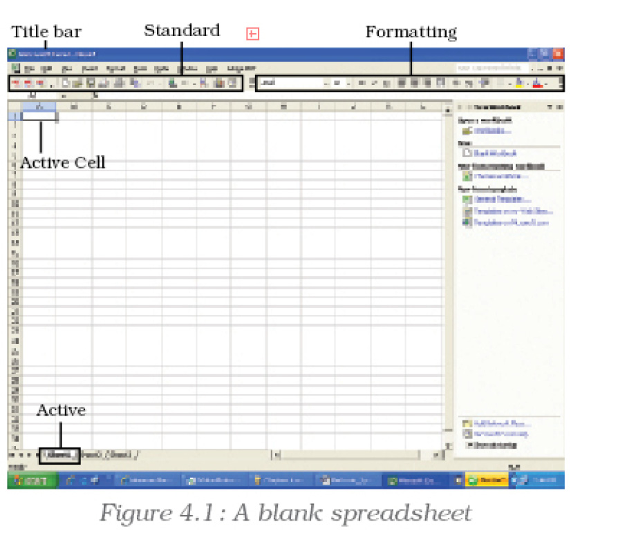
A blank spreadsheet as shown in figure 4.1 is displayed.
4.3 Basic Spreasdsheet Elements
4.3.1 Workbook and Worksheet
Each speadsheet file is known as a workbook and is stored with a default extension of .xls. Each workbook can contain many sheets, so various kinds of related information can be organised in a single file. Each workbook can contain up to 255 worksheets, but by default it displays only three. Worksheet is the area where the data is stored and work is performed. Extra worksheets can be added as and when required.
4.3.2 Rows, Columns and Cells
The rows in a worksheet are numbered from top to bottom along the left column of the worksheet. The columns are labeled from left to right with letters. The total number of rows in Excel are 65536 and the total number of columns are 256. Columns are named from A to IV. The rows are numbered from 1 to 65536.
A cell is the intersection of a row and a column. A cell is identified by an address that consists of the column name followed by the row number. For example, the first cell is referred to as A1, which indicates that it lies at the intersection of the column A and row 1. This is the active cell. The active cell is ready for accepting any action or input. A small group of contiguous cells is defined as a range. The range is referred to by writing the starting address of the cell in the range: Ending address of the cell in a range or vice versa. For example A1:A10 (can also be referred as A10 : A1).
4.4 Navigating in a Worksheet
The cursor keys, mouse and the scroll bar can be used to navigate through the worksheet. However, navigating through the 65,536 rows and 256 columns using these techniques is very inefficient. To move to any cell directly without scrolling through the entire worksheet, use any of the following shortcut methods:
Method 1 : Using key combinations
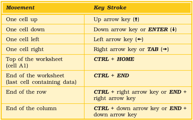
Method 2 : Using the name box
1. Type the cell address in the Name Box
2. Press ENTER to reach the desired cell.
For example, to move to cell D6, enter D6 in the Name Box and press
ENTER. The cursor is positioned on the cell in the D column and 6th row.
Method 3 : Using the go to dialog box
1. Press F5 or CTRL + G or choose Go To option from the Edit menu to invoke the Go To dialog box.
2. Enter the cell coordinates in the Reference textbox.
3. Click OK to move to the desired cell.
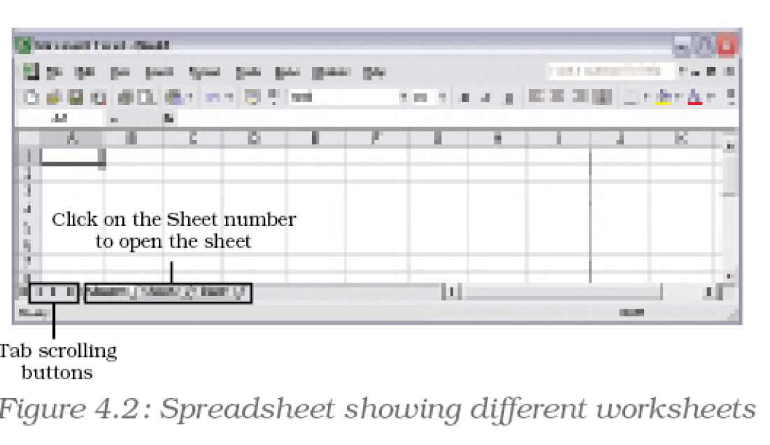
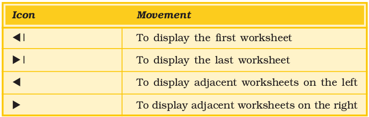
4.4.1 Navigating Between Worksheets
To move between worksheets, simply click on the sheet number in the lower left corner of the screen (Figure 4.2). In case the number of worksheets is more than the number which can be displayed use the tab scrolling buttons, located next to the sheet numbers and then click on the sheet number to select it.
The tab scrolling buttons and their use are given below:
4.5 Saving a Workbook
To save a Workbook:
1. Choose the Save As option from the File menu or Click on the Save button on the Standard Toolbar or Close the workbook by clicking on the Close button. The Save As dialog box is displayed as shown in the figure.
2. Select the directory in which the file is to be saved.
3. Type the name of the file in the File Name text box.
4. Click Save.
4.6 Opening a Workbook
To open a workbook:
1. Choose Open option from the File menu or Click on the Open button on the Standard Toolbar.
2. Select directory in which the file has been saved.
3. Type the name of the file in the File Name field or select the name by clicking on it.
4. Click Open.
4.7 Using Formulas and Functions
Formulas are entries containing an equation that calculates the value to be displayed. Please remember, when working with formulas, do not type in the numbers but type in the equation. This equation will be automatically updated upon the change or entry of any data that is referenced in the equation.
4.7.1 Entering Formulas
Cells in a worksheet can also contain formulas that are helpful in performing calculations. Formulas are mathematical equations. They are useful for establishing the relationship between two or more cells. They contain the coordinates of the cells that are used in the formula, operators and functions. When a formula is entered, the cell displays the result of the formula. Formulas must begin with an = sign, otherwise it is treated as a text entry (Figure 4.3).
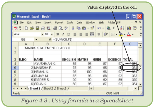
Whenever any cell value is changed it automatically recalculates the values of any formula and displays it in the relevant cell.
Using Arithmetic Operators
When a number is entered into a cell, it is possible to perform mathematical calculations using them. Spreadsheets have many mathematical functions built into them. The most basic operations used widely are addition, subtraction, multiplication and division. Follow the given steps to perform addition.
1. Move the cursor to cell A1. Type 1.
2. Press Enter to move to cell A2. Type 1 in cell A2.
3. Press Enter to move to cell A3.
4. Type =A1+A2 in cell A3.
Note that the contents of cell A1 and A2 have been added and the result is shown in cell A3 (Figure 4.4).
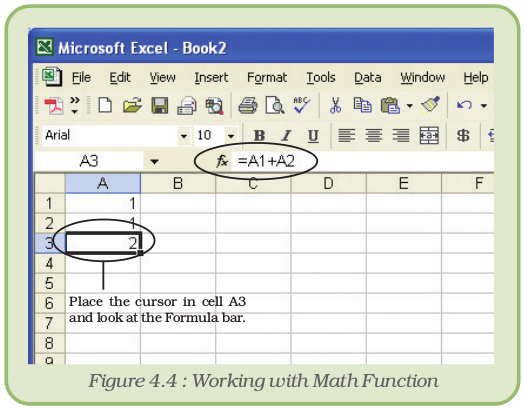
The same steps can be followed to perform other mathematical operations by simply changing the formula typed into cell A3.
Using Auto Sum
The addition of numbers is one of the most frequently used actions. Thus, a toolbar button, AutoSum, has been provided to accomplish this task. The AutoSum button on the Standard toolbar automatically adds the values above the destination cell or to the left of the destination cell. The steps to illustrate this are as follows:
1. Click on the destination cell i.e. the cell in which the result is to be displayed.
2. Click on the AutoSum button, which is located on the Standard toolbar. The cells containing the numbers to be added automatically should now be highlighted.
3. Press Enter to see the result in the destination cell.
4.7.2 Functions
This has a set of prewritten formulas called functions. Functions are special programs that accept data and return a value after processing the data. Functions differ from regular formulas because they accept values and not the operators, such as +, -, *, or /. For example, the SUM function can be used to add numbers in place of the ‘+’ operator. When using a function, remember the following :
- Use an equal to sign (=) to begin a formula.
- Specify the function name.
- Enclose arguments (data accepted by a function) within parentheses.
- Use a comma to separate arguments.
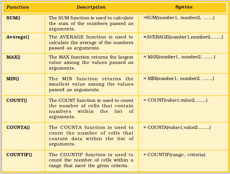
Some commonly used Functions are listed in Table representing some commonly used Functions (Appendix 4.1)
4.7.3 Copying and Pasting Formulas and Functions
Sometimes when working with formulas, the need arises to repeat the same formula for many different cells. The formulas can be copied using various methods.
Method 1 : Using the Edit menu
Steps are given below:
1. Click on the cell that contains the formula.
2. Choose the Copy option from the Edit menu.
3. Click on the cell where the formula is to be copied.
4. Choose the Paste option from the Edit menu. Note the change in the cell reference.
5. Press Esc to exit the Copy mode.
Method 2 : Using the Formatting Toolbar / Keyboard Shortcuts
Steps are given below :
1. Click on the cell that contains the formula.
2. Click on the Copy icon  located on the Formatting toolbar or press Ctrl + C keys.
3. Click on the cell where the formula is to be copied.
4. Click on the Paste icon  located on the Formatting toolbar or press Ctrl + V keys.
5. Press Esc to exit the Copy mode.
If a formula needs to be copied to multiple cells, use the AutoFill feature discussed later in the lesson.
4.7.4 Cell Referencing
Observe that when you copy and paste formulas, they are pasted relative to the position they are copied from. This is because of the way the formula treats the cell references. The cell coordinates in the formula are known as cell references. Two commonly used cell references are – Absolute and Relative.
Absolute Referencing
Absolute referencing implies that the coordinates of a cell are not changed when a formula is copied from one cell to another. To make a cell address an absolute cell address place a dollar sign in front of both the row and column identifiers. For example, $A$1 implies that both row and column have been fixed or made absolute. In simple words this means that while copying this formula to another cell, neither the column name nor the row number will change.
Relative Referencing
With relative cell referencing, when we copy a formula from one area of the worksheet to another, it records the position of the cell relative to the cell that originally contained the formula. This is the default mode of referencing in a spreadsheet.
The F4 key is used to toggle between the absolute and relative modes of referencing cells.
4.8 Working with Worksheet Ranges
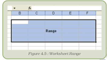
Each cell is referred to by a cell address. A group of cells are referenced using a reference operator. There are two types of reference operators, range and union.
- A range reference refers to all the cells between and including the reference (Figure 4.5). A range reference consists of two cell addresses separated by a colon. The range reference B1:B4 includes cells B1, B2, B3 and B4. The range reference A1:B3 includes A1, A2, A3, B1, B2 and B3.
- A union reference includes two or more references. A union reference consists of two or more cell addresses separated by a comma. For example, the reference A1, B5, C7 refers to cells A1, B5, and C7. Similarly, the reference A1:A3,B4:B6 refers to cells A1, A2, A3, B4, B5 and B6.
4.8.1 Using Range Names in Formulas
When working with large volumes of data in a worksheet, it is frequently desirable to refer to a range of cells repeatedly. For example, if a column in the worksheet contains the price of products, it will be required again and again for calculating the total price of all products or calculating the average price and so on. In such a case, it is convenient and efficient to name this range meaningfully and use the name of the range instead of the cell coordinates. Naming a range of cells has the following advantages:
- Names are easier to remember than cell coordinates.
- Names make navigation in a worksheet easier.
- Named ranges can be used throughout a workbook easily. This is very helpful while linking worksheets in a workbook.
4.8.2 Creating Range Names
Steps to create a named range are:
1. Select the cell or range of cells to be named.
2. Choose the Name option from the Insert menu.
3. Choose the Define option from the Name sub-menu. The Define Name dialog box is displayed as in figure 4.6.
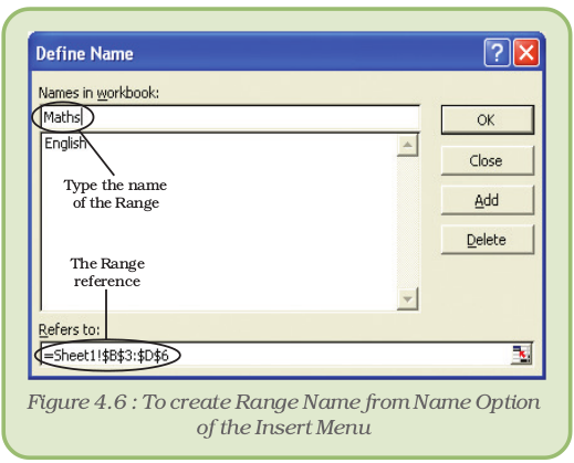
4. Type in the name of the range in the Names in a workbook text box.
5. Click on the Add button to create the name. The name is immediately added to the existing names in the box.
6. Click on the OK button to close the dialog box.
4.8.3 Using Range Names
Simply type the name in the formula in place of the cell coordinates. For example, to find the maximum of a range of marks named Maths, the formula will be =MAX(Maths).
4.9 Working with Rows And Columns
To add extra information to a worksheet, it may sometimes be desirable to insert new rows and columns. To insert a new row/ column, execute the following steps:
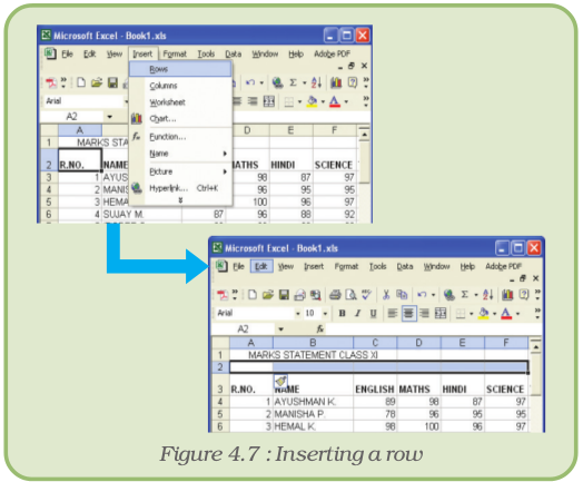
4.9.1 Inserting a Row
1. Click on the Row Number (or any cell in that row) above which the new row is to be added.
2. Choose the Rows option from the Insert menu. A row is inserted above the selected row (Figure 4.7).
3. Click any where in the spreadsheet to remove the selection.
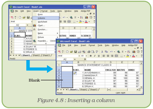
4.9.2 Inserting a Column
1. Click on the Column name (or any cell in that column).
2. Choose the Columns option from the Insert menu. A column is inserted to the left of the selected column (Figure 4.8).
3. Click anywhere in the spreadsheet to remove the selection.
4.9.3 Deleting Rows and Columns
When the contents of an entire row or column are to be deleted, perform the following steps:
1. Click on the Row Number/Column Name to be deleted.
2. Choose the Delete option from the Edit menu or right click and select Delete option from the pop-up menus.
3. Click anywhere in the spreadsheet to remove the selection.
4.9.4 Inserting and Deleting Cells
We can insert or delete individual cells also, rather than the entire row or column.
Inserting a Cell
1. Click on the cell where new cell(s) is to be inserted.
2. Choose the Cells option from the Insert menu. The Insert dialog box is displayed (Figure 4.9).
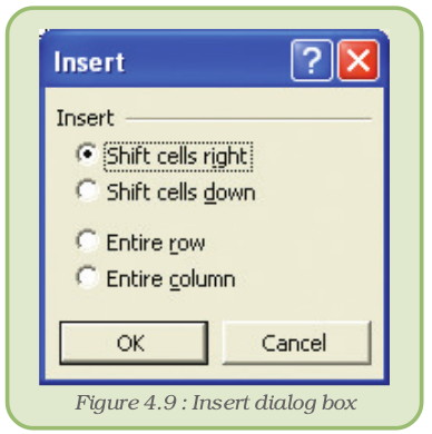
3. Choose the appropriate option. The result of each option is explained as under:
(a) Shift cells right – adds a blank cell to the left of the selected cell.
(b) Shift cells down – adds a blank cell above the selected cell.
(c) Entire row – adds a new row above the selected cell.
(d) Entire column – adds a new column to the left of the selected cell.
4. Click on OK button.
Deleting a Cell
1. Click on the cell which is to be deleted.
2. Choose the Delete option from the Edit menu. The Delete dialog box is displayed as shown in figure 4.10.
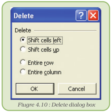
3. Choose the appropriate option. The result of each option is explained as under:
(a) Shift cells left – the cells to the right of the deleted cell are moved left.
(b) Shift cells up – the cells below the deleted cell are moved up.
(c) Entire row – deletes the entire row and moves the row below upwards.
(d) Entire column – deletes the entire column and moves the row to the right leftwards.
4. Click on OK button.
Note: If there is any data at the extreme right or at the end of the worksheet, it does not allow us to insert cells or rows. This is because, it does not delete existing contents from the worksheet while inserting cells. For example, if there is data in row number 16,384, then inserting a row will result in an error.
4.9.5 Clearing Data
To delete an entry in a cell or a group of cells, place the cursor in the cell or highlight the group of cells and press the Delete key. Note that this method only clears the cell contents and not the cell formats or comments.
Alternatively, use the Edit menu that allows an option of what to delete.
Steps for clearing data using Edit menu are as under:
1. Click on the cell or select the cell range whose contents are to be deleted.
2. Choose the Clear option from the Edit menu.
3. Choose the relevant option from the Clear sub-menu.
The Clear sub-menu offers four choices (Figure 4.11) explained as below:
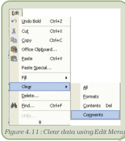
- All – to delete all formats, contents and comments.
- Formats – to delete formats only.
- Contents – to delete contents only.
- Comments – to delete comments only.
4.10 Selecting Cells
To perform a function on any particular cell or a group of cells, the cell or cells need to be first selected. Selecting a single cell is as simple as clicking on it.
4.10.1 Select a Row
To select an entire row, click on the row number to be selected on the left hand side of the spreadsheet.
4.10.2 Select a Column
To select an entire column, click on the column label at the top of the spreadsheet.
4.10.3 Select all Cells in a Worksheet
Click on the empty grey box in the left corner between A and 1. This area is called the Select All button.
4.10.4 To Select a Contiguous Group of Cells
To select adjacent cells, use any of the following methods.
Method 1 : Using the Name Box
1. Click on the Name Box.
2. Type the cell reference of the starting cell and the ending cell separated by a colon in the Name Box. For example, to select cells A3 to A10, type A3:A10 in the Name Box.
3. Press Enter to select the cells.
For example, as shown in the figure 4.12, typing A1:D1 in the Name Box selects the cells in the specified range i.e. A1,B1,C1,D1.
Figure 4.12 : Selecting Contiguous Group of Cells using Name Box
Method 2 : By Dragging
1. Place the cursor in the starting cell.
2. Holding down the left mouse button, drag the mouse over the area which is to be selected.
4.10.5 To Select Non–continuous Group of Cells
1. Place the cursor in cell A1.
2. Press the left mouse button.
3. While holding down the CTRL key and left mouse button, move mouse from starting cell to ending cell. Holding down the Ctrl key enables one to select non–contiguous areas of the worksheet.
4. Perform the desired operation or Press Esc and click anywhere on the worksheet to remove the highlighting.
4.11 Editing Cell Contents
After entering data into a cell, changes can be made to it using any of the following methods:
Method 1 : Using the F2 Key
1. Move the cursor to the desired cell whose contents have to be edited.
2. Press F2. Make the necessary changes.
3. Press Enter.
Method 2 : Using the Formula Bar
1. Move the cursor to the desired cell whose contents have to be edited.
2. Click in the formula area of the Formula Bar. (Figure 4.13)
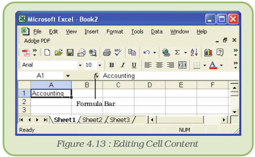
3. Make the necessary changes.
4. Press Enter.
Method 3 : Double-click in the Cell
1. Move the cursor to the desired cell whose contents have to be edited.
2. Double-click in the cell.
3. Make the necessary changes.
4. Press Enter.
4.12 Formatting Worksheets
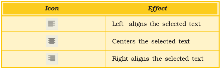
4.12.1 Aligning Cell Content
By default, text entries are left aligned and formulas and numbers are also left aligned. These alignments can be changed. Apart from the Left, Right and Center alignment options, the entries can be aligned vertically also. There are two methods for changing the horizontal cell alignment as explained below.
Method 1 : Using the Menu
1. Click on the cell to be aligned.
2. Choose the Cell option from the Format menu. The Format cells dialog box appears.
3. Choose the alignment tab.
4. Click to open the drop-down box associated with the horizontal field. After the drop-down box is opened, select the desired alignment as Right, Left or Center.
5. Click OK to close the dialog box.
Method 2 : Using the Format Toolbar
1. Click on the cell to be aligned.
2. Click on the appropriate alignment button in the Format toolbar to change the alignment.
To change the vertical alignment select the desired alignment as Center or Bottom from the Vertical drop-down box in the Format Cells dialog box displayed above.
Note : To make the line of data fit evenly within the height of a cell, choose the justify option.
4.12.2 Changing Column Width
There are two methods to change the column width.
Method 1 : Using the Menu Bar
1. Place the cursor anywhere in the column whose width is to be changed.
2. Choose the Column option from the Format menu. A dialog box opens.
3. Type in the required Column width in the dialog box and click on OK.
Method 2 : By Dragging
1. Place the cursor on the line between the B and C column headings. The cursor with two arrows appears.
2. Move the mouse to the right while holding down the left mouse button. The width indicator appears on the screen.
3. Release the left mouse button when the width indicator shows the desired width.
4.12.3 Changing Row Height
There are two methods to change the row height.
Method 1 : Using the Menubar
1. Place the cursor anywhere in the row whose height is to be changed.
2. Choose the Row option from the Format menu. A dialog box opens.
3. Type in the required Row Height in the dialog box and click on OK.
Method 2 : By Dragging
1. Place the cursor on the line between the 1 and 2 row headings. The cursor should look like the one displayed above, with two arrows.
2. Move the mouse downwards or upwards while holding down the left mouse button. The height indicator appears on the screen.
3. Release the left mouse button when the height indicator shows the desired height.
4.12.4 Changing Font Attributes
The Font style, size and colour can be easily changed in a spreadsheet to dress it up a little. To set the Font properties perform the following steps.
1. Click on the cell whose font properties are to be changed.
2. Choose the Cell option from the Format menu. The Format cells dialog box appears.
3. Choose the Font tab.
4. Change the Font type, style, size and colour using the appropriate options.
5. Click on OK.
Alternatively use the formatting tools available on the Formatting tool bar for changing the type, size and colour of the text.
4.12.5 Making Format Changes
Auto Formatting Worksheets
The Auto Format is a tool for creating pleasing worksheets with various formats quickly and easily. To Auto format a worksheet, follow the given steps:
1. Choose the Auto Format option from the Format menu.
2. Select the format to apply.
3. Click on OK.
Modifying Styles
The worksheet allows users to create, store and use individual formatting styles. A style can be defined as a collection of formats such as font size, patterns, and alignment that can be defined and saved as a group. To add or modify styles perform the following steps :
1. Choose Style option from the Format menu.
2. In the Style name box, type a name for a new style (Figure 4.14).
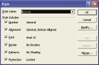
Figure 4.14 : Style option dialog box
3. To change formats for an existing style, click the style you want to change.
4. Click Modify.
5. On any of the tabs in the dialog box, select the formats you want, and then click OK.
6. Clear the check box for any type of formats that are not to be included in the style.
7. To define and apply the style to the selected cells, click OK.
8. To define the style without applying it, click Add, and then click Close.
Additional Formatting Options
Special Cell Borders
Another formatting feature, which can improve the readability of a spreadsheet, is to add borders around cells. This is especially useful if spreadsheet needs to be printed, because, by default, the light grey cell gridlines don’t appear when a spreadsheet document is printed.
To set borders, the steps are:
1. First select the cells on which you want to put borders.
2. Then click the Borders button on the toolbar at the top of the screen  .
.
3. Select a border style from the options that are displayed in figure 4.15. In the example below, the All Borders options is selected – this places a single line around all sides of all of the selected cells.
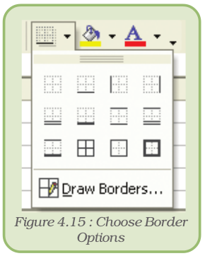
It is also possible to give different borders on different sides of a cell or have coloured borders around cells. Use the Draw borders option for this purpose. For this, follow the given steps:
1. Click on the down arrow next to the borders button  on the formatting Toolbar.
2. Select the Draw Borders option from the drop-down menu. The Borders toolbar is displayed as shown in figure 4.16.
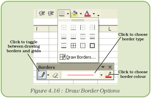
3. Choose the colour of the border and the type of the border and draw borders or grids.
Special Cell Shades
Cells can be filled with various colours or shading effects. For achieving this, use the Patterns tab of the Format cells menu. The steps to be followed are given below:
1. Select the cells to which cell shading is to be applied.
2. Choose the Cells option from the Format menu.
3. Click on the Patterns tab.
4. Choose the desired colour and/or pattern from the available list.
5. Click on OK.
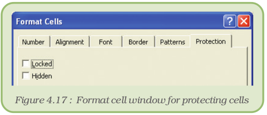
Protecting Cells
It allows us to set Protection options to prevent editing (or even viewing) of all or parts of a workbook. This can be very useful while sharing a spreadsheet with others or even to prevent accidental altering of labels and formulas once they are all completed.
It is necessary to set an option to unlock cells that may still require change after a worksheet is protected. By default every cell has its Locked property set to true. For unlocking cells :
1. Select the block of cells to be unlocked.
2. Choose the Cells option from the Format menu. The Format Cells window appears as shown in figure 4.18.
3. Click on the Protection tab.
4. Click in the box next to Locked to remove the check mark.
5. Click OK. The Locked property for these cells is now disabled.
Conditional Formatting
This feature allows the user to apply formats to cells that satisfy a predefined criterion.
To apply conditional formatting, perform the following steps:
1. Choose Conditional Formatting option from the Format menu.
2. In the Conditional Formatting dialog box (Figure 4.19) specify criteria using the various options.
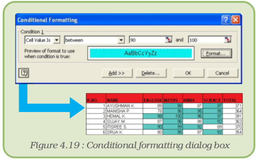
3. Click Format.
4. Select the font styles, borders, shading and other options to be applied.
5. Click OK to apply the formats to cells that meet the specified criterion.
Tab Colours
To separate out worksheets from one another, it is possible to give different colours to the name of the worksheets at the bottom left corner. The steps to be followed for achieving this are:
1. Click on the Sheet name.
2. Right click and in the pop up box choose the Tab Color option.
3. Select the desired colour from the Format Tab Color Dialog Box as shown in figure 4.20.
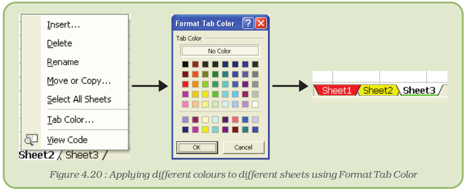
4. Click on OK to see the effect.
4.12.6 Using Charts
Charts are an excellent tool to present data in a worksheet in a visually appealing format which aids in analysing and comparing data. The Chart Wizard button  guides through the steps for creating an embedded chart. The steps are as follows:
1. Highlight all the cells that need to be included in the chart including headers.
2. Choose the Chart option from the Insert menu.
3. Choose the suitable Chart type from any of the available types. We will select Column. There are various types available like Pie Chart, Bar Chart, Line Chart, etc.
4. In the Chart Sub-type box, choose the Clustered Column icon to select the chart sub-type.
5. Click Next.
6. The next step displays the address of the cell range selected for preparing the chart. If the need arises, this range can be changed by clicking on the collapse dialog box.
7. Click Next.
8. To place the Subject data on the x-axis, select the Rows radio button.
9. Click Next.
10. Type Class XI Performance in the Chart Title textbox.
11. Type Subjects in the Category (X) Axis field. Subjects will appear as the x-axis title.
12. Type Marks in the Value (Y) Axis field. Marks will appear as the y-axis title.
13. Choose the Data Table tab.
14. Select Show Data Table if required.
15. Click Next.
16. Choose the As Object in Sheet1 option to make the chart an embedded object and part of the current worksheet. In case we need it on a new sheet, then we may choose the option As New Sheet.
17. Click Finish.
Activity
Let us explore it by ourselves creating a worksheet and using different Chart Options.
4.12.7 Using Special Tools
Spell Checking
The Spell Check feature of spreadsheet is same as that for Word Processing which we used in the previous chapter.
1. Select the range of cells to be checked.
2. Click on Spelling  button on the Standard Toolbar.
3. On locating an error, make changes accordingly.
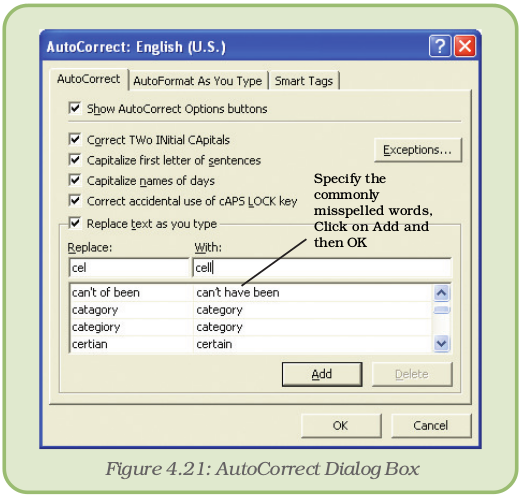
AutoCorrect Worksheets
The AutoCorrect feature can correct common typing errors during working. For example, it can change “adn” to “and” and change “their is” to “there is.” The commonly misspelt words can be added as an AutoCorrect entry (Figure 4.21). The common misspelling is then automatically corrected.
4.12.8 Finding and Replacing Data
This feature is useful in finding and replacing multiple occurrences of a value in the worksheet quickly and efficiently. The steps involved are as given below:
1. Click on the cell whose value is to be found and replaced.
2. Choose the Replace option from the Edit menu. The Find & Replace menu box opens (Figure 4.22).
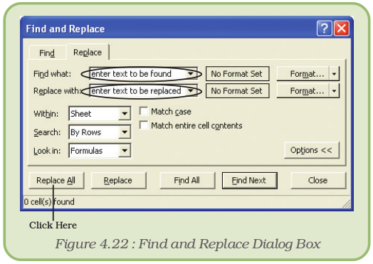
3. Enter the text to be found in the Find What textbox.
4. Enter the text to be replaced with in the Replace With textbox.
5. Click on the Replace All button and then Click on OK when prompted.
6. Click on Close to come out of the dialog box.
4.12.9 Using Autofill
Excel contains a feature called AutoFill, which copies a logical series of values, labels or formulas. The AutoFill handle, which is like the “+” mathematical operator, can be located at the bottom right corner of the active cell.
To fill series perform the following steps:
1. Click on the first cell and type in “01-May”.
2. Click on the cell again and then position the mouse in the bottom right of the cell so that the cursor turns to a small black plus sign, as shown below.
3. With the cursor, click, hold and drag the mouse down.
4. It automatically copies the date and increments by one day for each cell going down, giving the series 1-May, 2-May, ... , 10-May. It keeps showing exactly which day is being filled. Release the mouse when the desired date is reached (Figure 4.23).
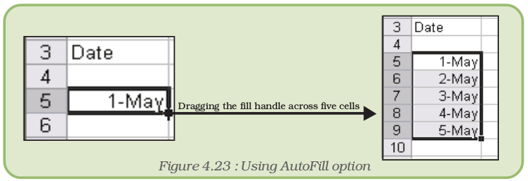
Note : Advanced options on creating such auto-fill series are available with the menu command Edit > Fill > Series.
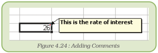
4.12.10 Adding Comments
Cell comments are additional explanatory notes which can be attached to a cell in a spreadsheet.
Cell comments are indicated by the small red triangle in the upper right corner of the cell. To view the comment, rest the pointer over the cell. A text box will appear, as shown in the figure 4.24.
To add a comment to a cell follow the given steps:
1. Click on the cell to which the comment is to be added.
2. Choose Comment from the Insert menu.
3. In the box, type the comment text.
4. Once the comment is typed, click outside the comment box. The comment disappears but a small red triangle appears at the top right corner of the cell.
To edit an existing cell comment, follow the given steps:
1. Click on the cell with the comment we want to edit.
2. On the Insert menu, click Edit Comment.
3. Edit the comment and click outside the comment box.
4.13 Printing a Worksheet/Workbook
The simplest way to print a workbook is to click the Print icon located on the Standard toolbar. Dotted lines will appear on the screen after clicking on the print icon. These dotted lines indicate the right, left, top, and bottom edges of the printed pages. Before the printing can be done, it offers a variety of options to customise the printing according to specific needs.
4.13.1 Print Preview
There are many print options. All Office packages offer a facility of previewing a worksheet before it is actually printed in order to customise the print according to one’s specific requirements. Print options can be selected using the Page Setup dialog box or in the Print Preview. In Print Preview, it is possible to see the results of selections onscreen.
4.13.2 Print a Spreadsheet
To print a spreadsheet:
1. Choose Print Preview option from the File menu or click on the Print icon in the Standard toolbar.
2. Click Setup.
3. Choose the Page tab (Figure 4.25).
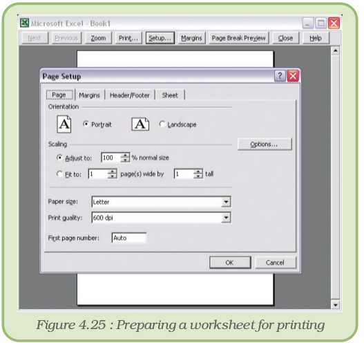
4. Choose Portrait or Landscape.
5. In the Adjust To field, type 100% to set the size to 100%.
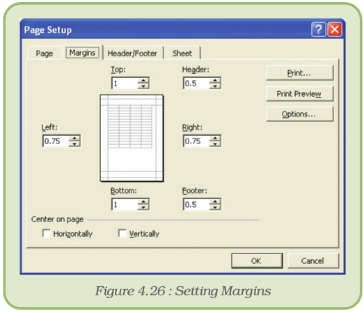
6. Choose the Margin tab.
7. Check the Horizontally box in the Center On Page frame to center the spreadsheet horizontally.
8. Click OK.
9. Click Print. The Print dialog box opens.
10. Click OK to print the file.
Summary
- A spreadsheet, also known as a worksheet, is a row and column arrangement of data and the formulas to manipulate the data.
- A spreadsheet can be used for a variety of applications like business forecasts, inventory control and accounting.
- Every Excel file is a workbook that can contain more than one worksheet.
- Cell is defined as the space where a specified row and a column intersect.
- Worksheets can contain labels, numbers or formulas.
- Worksheet allows selecting both contiguous and non-contiguous cells.
- A range is a group of cells referenced with a name. The range reference consists of the first and last cell addresses separated by a colon.
- The AutoSum button on the Standard toolbar adds numbers automatically and also suggests the range of numbers to be added.
- Formulas and functions are automatically updated with a change in the source cell or position of the formula.
- In Relative referencing, the reference is adjusted relative to the new location of the formula.
- In Absolute referencing, the cell reference does not change but remains fixed while pasting formulas.
- Functions are pre-written formulas which must begin with an “=” sign.
- Cell ranges can be named and used in place of cell references.
- The AutoFill handle is a very useful tool to fill in logical series.
- Cell comments are additional explanatory notes which can be attached to a cell in a spreadsheet.
- Charts are an excellent tool to present data graphically and also help in analysing and comparing data.
- The most powerful feature of a spreadsheet package is the “What-if analysis”. Using this feature, we can change values and immediately see the effect as the entire worksheet is automatically updated, based on the change in the values.
Exercise
Short Answer Type Questions
1. Define spreadsheet. Name any two spreadsheet software.
2. How many rows and columns are there in MS Excel?
3. How can you write a formula in Excel? Write a valid formula.
4. What is the shortcut to print current time in a cell?
5. Create a table to summarise the alignments of different types of datatype.
6. What is the use of auto correct option?
7. What is the use of print preview feature?
8. What is the use of auto sum feature?
9. How many function categories and functions are there in Excel? What do you understand by automatic recalculation feature of a spreadsheet?
10. Differentiate between relative and absolute cell referencing with the help of suitable examples.
11. Explain the uses of any two inbuilt mathematical functions in Excel.
12. Differentiate between the COUNT( ) and COUNTA( ) functions of Excel.
13. What is the function of the auto fill handle in Excel?
Long Answer Type Questions
1. What do you mean by conditional formatting? Explain.
2. Explain any five types of charts in Excel.
Multiple Choice Questions
1. A range refers to a  of cells.
(i) Row
(ii) Column
(iii) Group of contiguous cells
(iv) Group of non-contiguous cells
2. In  referencing, the cell reference does not change while copying formulas.
(i) Relative referencing
(ii) Absolute referencing
(iii) Mixed referencing
(iv) None of the above
3. Which of the following function keys is used as a toggle key for changing referencing modes?
(i) F2
(ii) F8
(iii) F4
(iv) F6
4. Which one of the following is the default folder for saving the files?
(i) c:\
(ii) d:\
(iii) my documents
(iv) new folder
5. A valid formula in Excel begins with:
(i) +
(ii) –
(iii) #
(iv) =
6. How many sheets are there in a workbook by default:
(i) 1
(ii) 2
(iii) 3
(iv) 4
7. Which function key is used to edit cell contents:
(i) F1
(ii) F2
(iii) F3
(iv) F4
8. Height of a row in Excel is:
(i) 12
(ii) 12.25
(iii) 12.50
(iv) 12.75.
Activities
Activity 4.1
Prepare an analytical result report of Second Monday Test Round Exam of your class in the format given below.
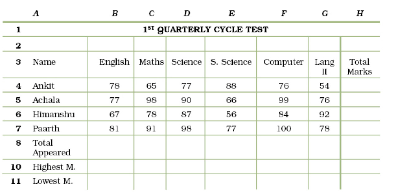
Instructions
- Calculate the total marks obtained by each student in column I.
- Calculate the highest and lowest marks obtained in each subject in row 9 and 10 respectively.
- Also calculate the aggregate/percentage marks obtained by each student in column J
- Give the number of students appearing for each subject in row11.
- Find the subject-wise average marks and display them in the row 8.
Activity 4.2
Prepare a score sheet of an inter-house cricket match in your school:
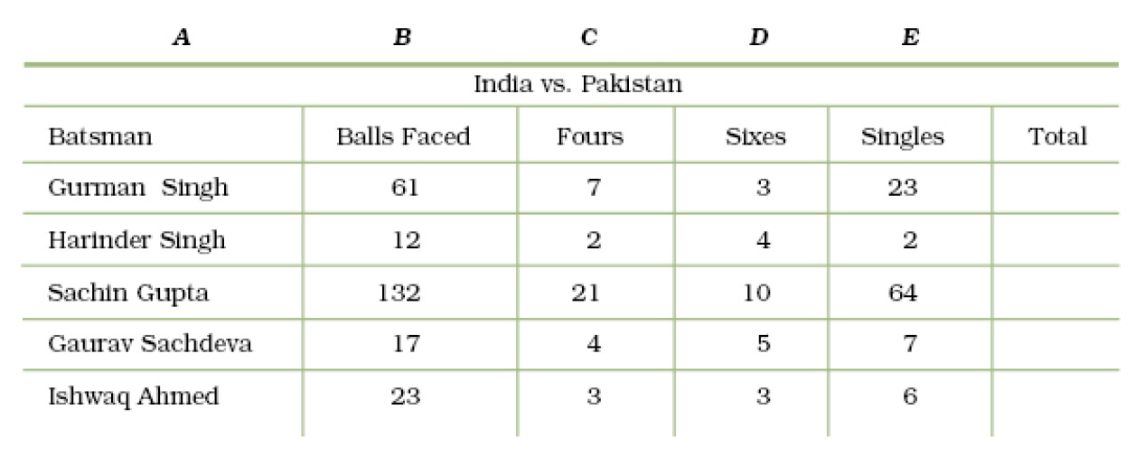
Instructions
- Calculate the total runs obtained by each student in column E.
- ( Total = No. of sixes x 6 + No. of fours x 4 + No. of Singles)
- Calculate the Strike Rate of each batsman in column F.
- Draw the pie chart to compare the strike rate of each batsman.
Activity 4.3
Prepare a personal expenditure report of last financial year in the format as below.
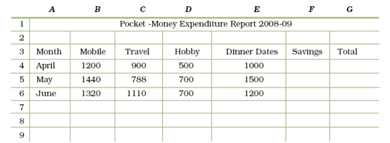
Instructions
- Assume that you are given a monthly pocket-money of Rs. 6000.
- Calculate the savings made by you every month.
- Calculate the total expenditure in each month.
- Calculate the highest and lowest expenditure made.
- Calculate the total savings after the three months
- Draw the bar graph to compare the expenditure of various months.
Activity 4.4
Prepare a report on purchase and sale of any 10 items of a shop over a week depicting the profit/loss in the format specified below.
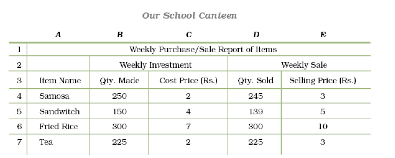
Instructions
- Calculate the total amount invested on each of the items. Total Amount Invested=Qty. Purchased * Cost price.
- Calculate the total selling price of each of the items. Total Selling Price=Qty. Sold * Selling Price.
- Calculate the Profit/Loss of each of the items. Profit/Loss =Total Selling Price-Total Amount Invested.
- Calculate the overall Profit/Loss made by Our School Canteen.
Appendix
Appendix 4.1 : Annexure – Table Representing Some Commonly Used Functions