Table of Contents

Chapter 15
STATISTICS
 “Statistics may be rightly called the science of averages and their
estimates.” - A.L.Bowley & A.L. Boddington
15.1 Introduction

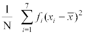
We know that statistics deals with data collected for specific purposes. We can make decisions about the data by analysing and interpreting it. In earlier classes, we have studied methods of representing data graphically and in tabular form. This representation reveals certain salient features or characteristics of the data. We have also studied the methods of finding a representative value for the given data. This value is called the measure of central tendency. Recall mean (arithmetic mean), median and mode are three measures of central tendency. A measure of central tendency gives us a rough idea where data points are centred. But, in order to make better interpretation from the data, we should also have an idea how the data are scattered or how much they are bunched around a measure of central tendency.
Batsman A : 30, 91, 0, 64, 42, 80, 30, 5, 117, 71
Batsman B : 53, 46, 48, 50, 53, 53, 58, 60, 57, 52
Clearly, the mean and median of the data are
Batsman A Batsman B
Mean 53 53
Median 53 53
Recall that, we calculate the mean of a data (denoted by  ) by dividing the sum of the observations by the number of observations, i.e.,

Also, the median is obtained by first arranging the data in ascending or descending order and applying the following rule.
If the number of observations is odd, then the median is 
 observation.
If the number of observations is even, then median is the mean of  and
and  observations.
We find that the mean and median of the runs scored by both the batsmen A and B are same i.e., 53. Can we say that the performance of two players is same? Clearly No, because the variability in the scores of batsman A is from 0 (minimum) to 117 (maximum). Whereas, the range of the runs scored by batsman B is from 46 to 60.
Let us now plot the above scores as dots on a number line. We find the following diagrams:
For batsman A

Fig 15.1
For batsman B

Fig 15.2
We can see that the dots corresponding to batsman B are close to each other and are clustering around the measure of central tendency (mean and median), while those corresponding to batsman A are scattered or more spread out.
Thus, the measures of central tendency are not sufficient to give complete information about a given data. Variability is another factor which is required to be studied under statistics. Like ‘measures of central tendency’ we want to have a single number to describe variability. This single number is called a ‘measure of dispersion’. In this Chapter, we shall learn some of the important measures of dispersion and their methods of calculation for ungrouped and grouped data.
15.2 Measures of Dispersion
The dispersion or scatter in a data is measured on the basis of the observations and the types of the measure of central tendency, used there. There are following measures of dispersion:
(i) Range, (ii) Quartile deviation, (iii) Mean deviation, (iv) Standard deviation.
In this Chapter, we shall study all of these measures of dispersion except the quartile deviation.
15.3 Range
Recall that, in the example of runs scored by two batsmen A and B, we had some idea of variability in the scores on the basis of minimum and maximum runs in each series. To obtain a single number for this, we find the difference of maximum and minimum values of each series. This difference is called the ‘Range’ of the data.
In case of batsman A, Range = 117 – 0 = 117 and for batsman B, Range = 60 – 46 = 14. Clearly, Range of A > Range of B. Therefore, the scores are scattered or dispersed in case of A while for B these are close to each other.
Thus, Range of a series = Maximum value – Minimum value.
The range of data gives us a rough idea of variability or scatter but does not tell about the dispersion of the data from a measure of central tendency. For this purpose, we need some other measure of variability. Clearly, such measure must depend upon the difference (or deviation) of the values from the central tendency.
The important measures of dispersion, which depend upon the deviations of the observations from a central tendency are mean deviation and standard deviation. Let us discuss them in detail.
15.4 Mean Deviation
Recall that the deviation of an observation x from a fixed value ‘a’ is the difference x – a. In order to find the dispersion of values of x from a central value ‘a’ , we find the deviations about a. An absolute measure of dispersion is the mean of these deviations. To find the mean, we must obtain the sum of the deviations. But, we know that a measure of central tendency lies between the maximum and the minimum values of the set of observations. Therefore, some of the deviations will be negative and some positive. Thus, the sum of deviations may vanish. Moreover, the sum of the deviations from mean (x) is zero.
(Also Mean of deviations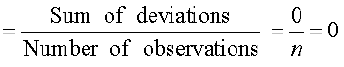 )
)
Thus, finding the mean of deviations about mean is not of any use for us, as far as the measure of dispersion is concerned.
Remember that, in finding a suitable measure of dispersion, we require the distance of each value from a central tendency or a fixed number ‘a’. Recall, that the absolute value of the difference of two numbers gives the distance between the numbers when represented on a number line. Thus, to find the measure of dispersion from a fixed number ‘a’ we may take the mean of the absolute values of the deviations from the central value. This mean is called the ‘mean deviation’. Thus mean deviation about a central value ‘a’ is the mean of the absolute values of the deviations of the observations from ‘a’. The mean deviation from ‘a’ is denoted as M.D. (a). Therefore,
M.D.(a)=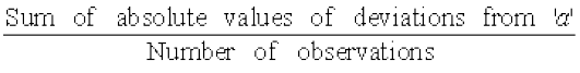
Remark Mean deviation may be obtained from any measure of central tendency. However, mean deviation from mean and median are commonly used in statistical studies.
Let us now learn how to calculate mean deviation about mean and mean deviation about median for various types of data
15.4.1 Mean deviation for ungrouped data
Let n observations be x1, x2, x3, ...., xn. The following steps are involved in the calculation of mean deviation about mean or median:
Step 1 Calculate the measure of central tendency about which we are to find the mean deviation. Let it be ‘a’.
Step 2 Find the deviation of each xi from a, i.e., x1 – a, x2 – a, x3 – a,. . . , xn– a
Step 3 Find the absolute values of the deviations, i.e., drop the minus sign (–), if it is there, i.e.,
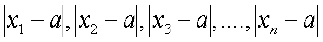 .
.
Step 4 Find the mean of the absolute values of the deviations. This mean is the mean deviation about a, i.e., 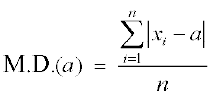
Thus M.D. ( 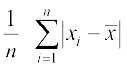 ) =
) = , where= Mean
and M.D. (M) = 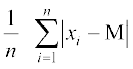 , where M = Median
Note In this Chapter, we shall use the symbol M to denote median unless stated otherwise.Let us now illustrate the steps of the above method in following examples.
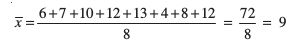
Example 1 Find the mean deviation about the mean for the following data:
6, 7, 10, 12, 13, 4, 8, 12
Solution We proceed step-wise and get the following:
Step 1 Mean of the given data is
Step 2 The deviations of the respective observations from the mean  i.e., xi–
 are
are
6 – 9, 7 – 9, 10 – 9, 12 – 9, 13 – 9, 4 – 9, 8 – 9, 12 – 9,
or –3, –2, 1, 3, 4, –5, –1, 3
Step 3 The absolute values of the deviations, i.e.,  are
are
3, 2, 1, 3, 4, 5, 1, 3
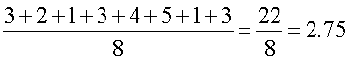
Step 4 The required mean deviation about the mean is
M.D.= 
= 
Note Instead of carrying out the steps every time, we can carry on calculation, step-wise without referring to steps.
Example 2 Find the mean deviation about the mean for the following data :
12, 3, 18, 17, 4, 9, 17, 19, 20, 15, 8, 17, 2, 3, 16, 11, 3, 1, 0, 5
Solution We have to first find the mean () of the given data
( )=
)= = 10
= 10
The respective absolute values of the deviations from mean, i.e., are
are
2, 7, 8, 7, 6, 1, 7, 9, 10, 5, 2, 7, 8, 7, 6, 1, 7, 9, 10, 5
Therefore 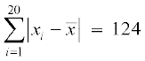
and M.D.()= = 6.2
= 6.2
Example 3 Find the mean deviation about the median for the following data:
3, 9, 5, 3, 12, 10, 18, 4, 7, 19, 21.
Solution Here the number of observations is 11 which is odd. Arranging the data into ascending order, we have 3, 3, 4, 5, 7, 9, 10, 12, 18, 19, 21
Now Median =  or 6th observation = 9
The absolute values of the respective deviations from the median, i.e., are
are
6, 6, 5, 4, 2, 0, 1, 3, 9, 10, 12
Therefore 
and 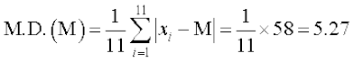
15.4.2 Mean deviation for grouped data We know that data can be grouped into two ways :
(a) Discrete frequency distribution,
(b) Continuous frequency distribution.
Let us discuss the method of finding mean deviation for both types of the data.
(a) Discrete frequency distribution Let the given data consist of n distinct values x1, x2, ..., xn occurring with frequencies f1, f2 , ..., fn respectively. This data can be represented in the tabular form as given below, and is called discrete frequency distribution:
x : x1 x2 x3 ... xn
f : f1 f2 f3 ... fn
(i) Mean deviation about mean
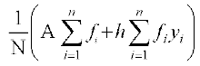
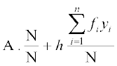
First of all we find the mean of the given data by using the formula

where  , denotes the sum of the products of observations xi with their respective frequencies fi and
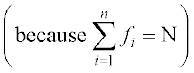
 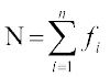 is the sum of the frequencies.
Then, we find the deviations of observations xi from the mean  and take their absolute values, i.e.,
  for all i =1, 2,..., n.
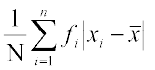
After this, find the mean of the absolute values of the deviations, which is the required mean deviation about the mean. Thus
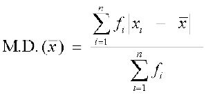 =
= 
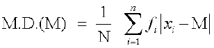
(ii) Mean deviation about median To find mean deviation about median, we find the median of the given discrete frequency distribution. For this the observations are arranged in ascending order. After this the cumulative frequencies are obtained. Then, we identify the observation whose cumulative frequency is equal to or just greater than  , where N is the sum of frequencies. This value of the observation lies in the middle of the data, therefore, it is the required median. After finding median, we obtain the mean of the absolute values of the deviations from median.Thus,
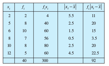
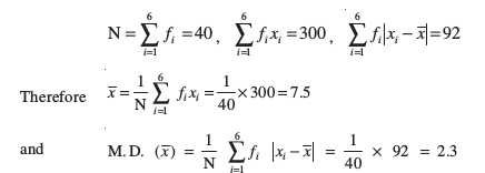
Example 4 Find mean deviation about the mean for the following data :
xi 2 5 6 8 10 12
fi 2 8 10 7 8 5
Solution Let us make a Table 15.1 of the given data and append other columns after calculations.
Table 15.1
Example 5 Find the mean deviation about the median for the following data:
| xi | 3 | 6 | 9 | 12 | 13 | 15 | 21 | 22 |
| fi | 3 | 4 | 5 | 2 | 4 | 5 | 4 | 3 |
Solution The given observations are already in ascending order. Adding a row corresponding to cumulative frequencies to the given data, we get (Table 15.2).
Table 15.2
| xi | 3 | 6 | 9 | 12 | 13 | 15 | 21 | 22 |
| fi | 3 | 4 | 5 | 2 | 4 | 5 | 4 | 3 |
| c.f. | 3 | 7 | 12 | 14 | 18 | 23 | 27 | 30 |
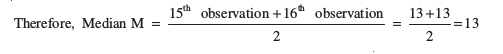
Now, N=30 which is even.
Median is the mean of the 15th and 16th observations. Both of these observations lie in the cumulative frequency 18, for which the corresponding observation is 13.
Now, absolute values of the deviations from median, i.e., are shown in Table 15.3.
Table 15.3
| 10 | 7 | 4 | 1 | 0 | 2 | 8 | 9 |
| fi | 3 | 4 | 5 | 2 | 4 | 5 | 4 | 3 |
| fi | 30 | 28 | 20 | 2 | 0 | 10 | 32 | 27 |
We have 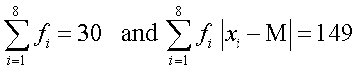
Therefore 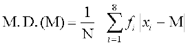
= 
= 4.97.
(b) Continuous frequency distribution A continuous frequency distribution is a series in which the data are classified into different class-intervals without gaps alongwith their respective frequencies.
For example, marks obtained by 100 students are presented in a continuous frequency distribution as follows :
| Marks obtained | 0-10 | 10-20 | 20-30 | 30-40 | 40-50 | 50-60 |
| Number of Students | 12 | 18 | 27 | 20 | 17 | 6 |
(i) Mean deviation about mean While calculating the mean of a continuous frequency distribution, we had made the assumption that the frequency in each class is centred at its mid-point. Here also, we write the mid-point of each given class and proceed further as for a discrete frequency distribution to find the mean deviation.
Let us take the following example.
Example 6 Find the mean deviation about the mean for the following data.
| Marks obtained | 10-20 | 20-30 | 30-40 | 40-50 | 50-60 | 60-70 | 70-80 |
| Number of students | 2 | 3 | 8 | 14 | 8 | 3 | 2 |
Solution We make the following Table 15.4 from the given data :
Table 15.4
| Marks obtained | Number of students fi | Mid-points xi | fixi | | fi |
| 10-20 20-30 30-40 40-50 50-60 60-70 70-80 | 2 3 8 14 8 3 2 | 15 25 35 45 55 65 75 | 30 75 280 630 440 195 150 | 30 20 10 0 10 20 30 | 60 60 80 0 80 60 60 |
| 40 | 1800 | 400 |
Here 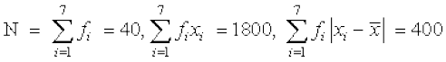
Therefore 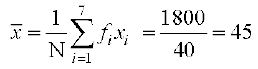
and 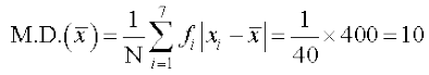
Shortcut method for calculating mean deviation about mean We can avoid the tedious calculations of computing 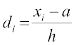 by following step-deviation method. Recall that in this method, we take an assumed mean which is in the middle or just close to it in the data. Then deviations of the observations (or mid-points of classes) are taken from the assumed mean. This is nothing but the shifting of origin from zero to the assumed mean on the number line, as shown in Fig 15.3
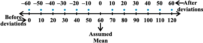
Fig 15.3
If there is a common factor of all the deviations, we divide them by this common factor to further simplify the deviations. These are known as step-deviations. The process of taking step-deviations is the change of scale on the number line as shown in Fig 15.4
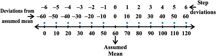
Fig 15.4
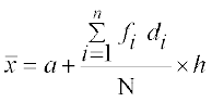
The deviations and step-deviations reduce the size of the observations, so that the computations viz. multiplication, etc., become simpler. Let, the new variable be denoted by  , where ‘a’ is the assumed mean and h is the common factor. Then, the mean by step-deviation method is given by
Let us take the data of Example 6 and find the mean deviation by using step-deviation method.
Take the assumed mean a = 45 and h = 10, and form the following Table 15.5.
Table 15.5
| Marks obtained | Number of students | Mid-points | 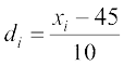 |  |  | fi |
| 10-20 20-30 30-40 40-50 50-60 70-80 | fi 2 3 8 14 8 3 2 | xi 15 25 35 45 55 65 75 | -3 -2 -1 0 1 2 3 | -6 -6 -8 0 8 6 6 | 30 20 10 0 10 20 30 | 60 60 80 0 80 60 60 |
| 40 | 0 | 400 |
Therefore 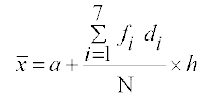
=
and 
. Rest of the procedure is same.(ii) Mean deviation about median The process of finding the mean deviation about median for a continuous frequency distribution is similar as we did for mean deviation about the mean. The only difference lies in the replacement of the mean by median while taking deviations.
Let us recall the process of finding median for a continuous frequency distribution.
The data is first arranged in ascending order. Then, the median of continuous frequency distribution is obtained by first identifying the class in which median lies (median class) and then applying the formula
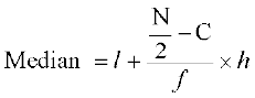
where median class is the class interval whose cumulative frequency is just greater than or equal to  , N is the sum of frequencies, l, f, h and C are, respectively the lower limit , the frequency, the width of the median class and C the cumulative frequency of the class just preceding the median class. After finding the median, the absolute values of the deviations of mid-point xi of each class from the median i.e., are obtained.
Then 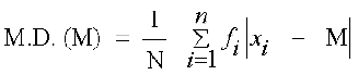
The process is illustrated in the following example:
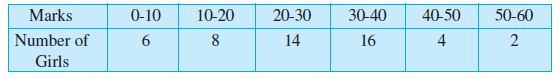
Example 7 Calculate the mean deviation about median for the following data :
| Class | 0-10 | 10-20 | 20-30 | 30-40 | 40-50 | 50-60 |
| Frequency | 6 | 7 | 15 | 16 | 4 | 2 |
Solution Form the following Table 15.6 from the given data :
Table 15.6
| Class | Frequency | Cumulative Frequency | Mid-points |  | fi |
| 0-10 10-20 20-30 30-40 40-50 50-60 | fi 6 7 15 16 4 2 | (c.f.) 6 13 28 44 48 50 | xi 5 15 25 35 45 55 | 23 13 3 7 17 27 | 138 91 45 112 68 54 |
| 50 | 508 |
The class interval containing  or 25th item is 20-30. Therefore, 20–30 is the median class. We know that
Median = 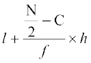
Therefore, Median = 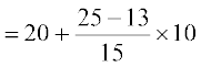 =20 + 8 = 28
Thus, Mean deviation about median is given by
M.D. (M) =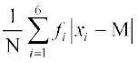 =
= = 10.16
Exercise15.1
Find the mean deviation about the mean for the data in Exercises 1 and 2.
1. 4, 7, 8, 9, 10, 12, 13, 17
2. 38, 70, 48, 40, 42, 55, 63, 46, 54, 44
Find the mean deviation about the median for the data in Exercises 3 and 4.
3. 13, 17, 16, 14, 11, 13, 10, 16, 11, 18, 12, 17
4. 36, 72, 46, 42, 60, 45, 53, 46, 51, 49
Find the mean deviation about the mean for the data in Exercises 5 and 6.
5. xi 5 10 15 20 25
fi 7 4 6 3 5
6. xi 10 30 50 70 90
fi 4 24 28 16 8
Find the mean deviation about the median for the data in Exercises 7 and 8.
7. xi 5 7 9 10 12 15
fi 8 6 2 2 2 6
8. xi 15 21 27 30 35
fi 3 5 6 7 8
Find the mean deviation about the mean for the data in Exercises 9 and 10.
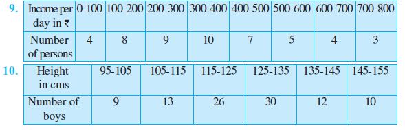
11. Find the mean deviation about median for the following data :
12. Calculate the mean deviation about median age for the age distribution of 100 persons given below:
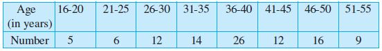
[Hint Convert the given data into continuous frequency distribution by subtracting 0.5 from the lower limit and adding 0.5 to the upper limit of each class interval]
15.4.3 Limitations of mean deviation In a series, where the degree of variability is very high, the median is not a representative central tendency. Thus, the mean deviation about median calculated for such series can not be fully relied.
The sum of the deviations from the mean (minus signs ignored) is more than the sum of the deviations from median. Therefore, the mean deviation about the mean is not very scientific.Thus, in many cases, mean deviation may give unsatisfactory results. Also mean deviation is calculated on the basis of absolute values of the deviations and therefore, cannot be subjected to further algebraic treatment. This implies that we must have some other measure of dispersion. Standard deviation is such a measure of dispersion.
15.5 Variance and Standard Deviation
Recall that while calculating mean deviation about mean or median, the absolute values of the deviations were taken. The absolute values were taken to give meaning to the mean deviation, otherwise the deviations may cancel among themselves.
Another way to overcome this difficulty which arose due to the signs of deviations, is to take squares of all the deviations. Obviously all these squares of deviations are non-negative. Let x1, x2, x3, ..., xn be n observations and be their mean. Then
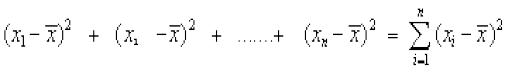
If this sum is zero, then each has to be zero. This implies that there is no dispersion at all as all observations are equal to the mean
If  is small , this indicates that the observations x1, x2, x3,...,xn are close to the mean and therefore, there is a lower degree of dispersion. On the contrary, if this sum is large, there is a higher degree of dispersion of the observations from the mean . Can we thus say that the sum is a reasonable indicator of the degree of dispersion or scatter?
Let us take the set A of six observations 5, 15, 25, 35, 45, 55. The mean of the observations is= 30. The sum of squares of deviations from for this set is
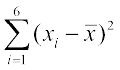 = (5–30)2 + (15–30)2 + (25–30)2 + (35–30)2 + (45–30)2 +(55–30)2
= 625 + 225 + 25 + 25 + 225 + 625 = 1750
Let us now take another set B of 31 observations 15, 16, 17, 18, 19, 20, 21, 22, 23, 24, 25, 26, 27, 28, 29, 30, 31, 32, 33, 34, 35, 36, 37, 38, 39, 40, 41, 42, 43, 44, 45. The mean of these observations is  = 30
= 30
Note that both the sets A and B of observations have a mean of 30.
Now, the sum of squares of deviations of observations for set B from the mean  is given by
 = (15–30)2 +(16–30)2 + (17–30)2 + ...+ (44–30)2 +(45–30)2
= (–15)2 +(–14)2 + ...+ (–1)2 + 02 + 12 + 22 + 32 + ...+ 142 + 152
= 2 [152 + 142 + ... + 12]
=  = 5 × 16 × 31 = 2480
(Because sum of squares of first n natural numbers = . Here n = 15)
If is simply our measure of dispersion or scatter about mean, we will tend to say that the set A of six observations has a lesser dispersion about the mean than the set B of 31 observations, even though the observations in set A are more scattered from the mean (the range of deviations being from –25 to 25) than in the set B (where the range of deviations is from –15 to 15).
This is also clear from the following diagrams.
For the set A, we have
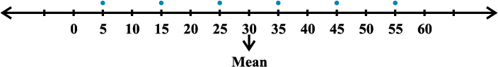
Fig 15.5
For the set B, we have
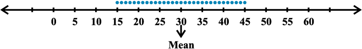
Fig 15.6
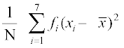
Thus, we can say that the sum of squares of deviations from the mean is not a proper measure of dispersion. To overcome this difficulty we take the mean of the squares of the deviations, i.e., we take 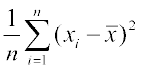 . In case of the set A, we have
 × 1750 = 291.67 and in case of the set B, it is
  × 2480 = 80.
This indicates that the scatter or dispersion is more in set A than the scatter or dispersion in set B, which confirms with the geometrical representation of the two sets.
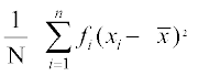
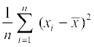
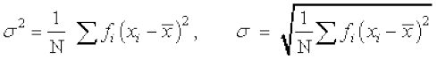
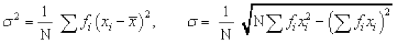
Thus, we can take 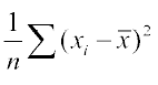 as a quantity which leads to a proper measure of dispersion. This number, i.e., mean of the squares of the deviations from mean is called the variance and is denoted by
  (read as sigma square). Therefore, the variance of n observations x1, x2,..., xn is given by
15.5.1 Standard Deviation
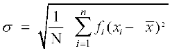
In the calculation of variance, we find that the units of individual observations xi and the unit of their mean are different from that of variance, since variance involves the sum of squares of (xi–). For this reason, the proper measure of dispersion about the mean of a set of observations is expressed as positive square-root of the variance and is called standard deviation. Therefore, the standard deviation, usually denoted by  , is given by
 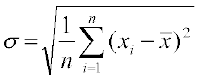 ... (1)
Let us take the following example to illustrate the calculation of variance and hence, standard deviation of ungrouped data.
Example 8 Find the variance of the following data:
6, 8, 10, 12, 14, 16, 18, 20, 22, 24
Solution From the given data we can form the following Table 15.7. The mean is calculated by step-deviation method taking 14 as assumed mean. The number of observations is n = 10
Table 15.7
| xi | 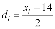 | Deviations from mean (xi– ) | (xi–) |
6 8 10 12 14 16 18 20 22 24 | -4 -3 -2 -1 0 1 2 3 4 5 | -9 -7 -5 -1 1 3 5 7 9 | 81 49 25 9 1 1 9 25 49 81 |
| 5 | 330 |
Therefore Mean = assumed mean + =
= 
and Variance ( ) =(
) =( ) =
) =  = = 33
Thus Standard deviation( ) (
) ( )
)
15.5.2 Standard deviation of a discrete frequency distribution
Let the given discrete frequency distribution be
x : x1, x2, x3 ,. . . , xn
f : f1, f2, f3 ,. . . , fn
In this case standard deviation 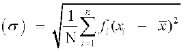 ... (2)
where  .
.
Let us take up following example.
Example 9 Find the variance and standard deviation for the following data:
| xi | 4 | 8 | 11 | 17 | 20 | 24 | 32 |
| fi | 3 | 5 | 9 | 5 | 4 | 3 | 1 |
Solution Presenting the data in tabular form (Table 15.8), we get
Table 15.8
| xi | fi | fi xi | xi – |  | fi |
| 4 8 11 17 20 24 32 | 3 5 9 5 4 3 1 | 12 40 99 85 80 72 32 | -10 -6 -3 3 6 10 18 | 100 36 9 9 36 100 324 | 300 180 81 45 144 300 324 |
| 30 | 420 | 1374 |
N = 30, 
Therefore 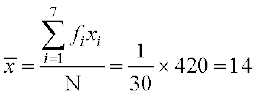
Hence variance  =
= =
=
=  × 1374 = 45.8
and Standard deviation  = 6.77
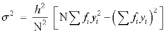
15.5.3 Standard deviation of a continuous frequency distribution
The given continuous frequency distribution can be represented as a discrete frequency distribution by replacing each class by its mid-point. Then, the standard deviation is calculated by the technique adopted in the case of a discrete frequency distribution.
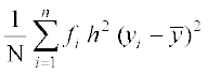
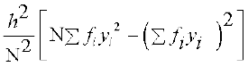
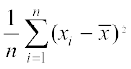
If there is a frequency distribution of n classes each class defined by its mid-point xi with frequency fi, the standard deviation will be obtained by the formula
where is the mean of the distribution and .
Another formula for standard deviation We know that
Variance =
= =
=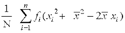
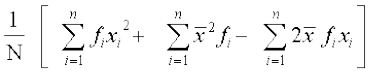
= 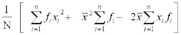
= 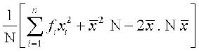
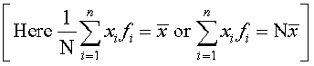
=
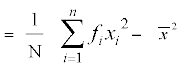
or  =
= 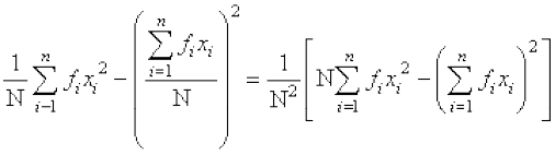
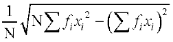
Thus, standard deviation 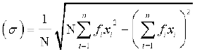 ... (3)
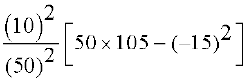
Example 10 Calculate the mean, variance and standard deviation for the following distribution :
| Class | 30-40 | 40-50 | 50-60 | 60-70 | 70-80 | 80-90 | 90-100 |
| Frequency | 3 | 7 | 12 | 15 | 8 | 3 | 2 |
Solution From the given data, we construct the following Table 15.9.
Table 15.9
| Class | Frequency (fi) | Mid-point (xi) | fixi | (xi–)2 | fi(xi–)2 |
| 30-40 40-50 50-60 60-70 70-80 80-90 90-100 | 3 7 12 15 8 3 2 | 35 45 55 65 75 85 95 | 105 315 660 975 600 255 190 | 729 289 49 9 169 529 1089 | 2187 2023 588 135 1352 1587 2178 |
| 50 | 3100 | 10050 |
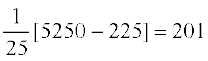
Thus 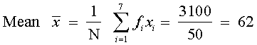
Variance 
=  = 201
= 201
and Standard deviation
Example 11 Find the standard deviation for the following data :
| xi | 3 | 8 | 13 | 18 | 23 |
| fi | 7 | 10 | 15 | 10 | 6 |
Solution Let us form the following Table 15.10:
| xi | fi | fixi | xi2 | fixi2 |
| 3 8 13 18 23 | 7 10 15 10 6 | 21 80 195 180 138 | 9 64 169 324 529 | 63 640 2535 3240 3174 |
| 48 | 614 | 9652 |
Now, by formula (3), we have
=
= 
= 
= 
= 6.12
Therefore, Standard deviation () = 6.12
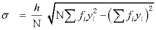
15.5.4. Shortcut method to find variance and standard deviation
Sometimes the values of xi in a discrete distribution or the mid points xi of different classes in a continuous distribution are large and so the calculation of mean and variance becomes tedious and time consuming. By using step-deviation method, it is possible to simplify the procedure.
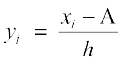
Let the assumed mean be ‘A’ and the scale be reduced to times (h being the width of class-intervals). Let the step-deviations or the new values be yi.
i.e.  or xi = A + hyi ... (1)
We know that  ... (2)
Replacing xi from (1) in (2), we get
 =
=
= 
= 
=
Thus = A + h ... (3)
Now Variance of the variable x,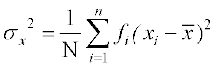
=  (Using (1) and (3))
= 
= 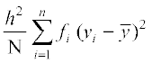 = h2 × variance of the variable yi
i.e.  =
= 
or 
 ... (4)
From (3) and (4), we have
=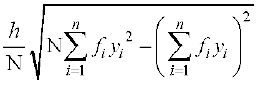 ... (5)
Let us solve Example 11 by the short-cut method and using formula (5)
Examples 12 Calculate mean, variance and standard deviation for the following distribution.
| Classes | 30-40 | 40-50 | 50-60 | 60-70 | 70-80 | 80-90 | 90-100 |
| Frequency | 3 | 7 | 12 | 15 | 8 | 3 | 2 |
Solution Let the assumed mean A = 65. Here h = 10
We obtain the following Table 15.11 from the given data :
Table 15.11
| Class | Frequency | Mid-point | yi= | yi2 | fi yi | fi yi2 |
| 30-40 40-50 50-60 60-70 70-80 80-90 90-100 | fi 3 7 12 15 8 3 2 | xi 35 45 55 65 75 85 95 | -3 -2 -1 0 1 2 3 | 9 4 1 0 1 4 9 | -9 -14 -12 0 8 6 6 | 27 28 12 0 8 12 18 |
| N=50 | – 15 | 105 |
Therefore  =
=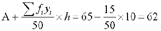 =
=
Variance  =
=
= 
= 
and standard deviation 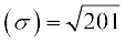 = 14.18
Exercise 15.2
Find the mean and variance for each of the data in Exercies 1 to 5.
1. 6, 7, 10, 12, 13, 4, 8, 12
2. First n natural numbers
3. First 10 multiples of 3
4.
| xi | 6 | 10 | 14 | 18 | 24 | 28 | 30 |
| fi | 2 | 4 | 7 | 12 | 8 | 4 | 3 |
5.
| xi | 92 | 93 | 97 | 98 | 102 | 104 | 109 |
| fi | 3 | 2 | 3 | 2 | 6 | 3 | 3 |
6. Find the mean and standard deviation using short-cut method.
| xi | 60 | 61 | 62 | 63 | 64 | 65 | 66 | 67 | 68 |
| fi | 2 | 1 | 12 | 29 | 25 | 12 | 10 | 4 | 5 |
Find the mean and variance for the following frequency distributions in Exercises 7 and 8.
7.
| Classes | 0-30 | 30-60 | 60-90 | 90-120 | 120-150 | 150-180 | 180-210 |
| Frequencies | 2 | 3 | 5 | 10 | 3 | 5 | 2 |
8.
| Classes | 0-10 | 10-20 | 20-30 | 30-40 | 40-50 |
| Frequencies | 5 | 8 | 15 | 16 | 6 |
9. Find the mean, variance and standard deviation using short-cut method
| Height in cms | 70-75 | 75-80 | 80-85 | 85-90 | 90-95 | 95-100 | 100-105 | 105-110 | 110-115 |
| No. of children | 3 | 4 | 7 | 7 | 15 | 9 | 6 | 6 | 3 |
10. The diameters of circles (in mm) drawn in a design are given below:
| Diameters | 33-36 | 37-40 | 41-44 | 45-48 | 49-52 |
| No. of circles | 15 | 17 | 21 | 22 | 25 |
[ Hint First make the data continuous by making the classes as 32.5-36.5, 36.5-40.5, 40.5-44.5, 44.5 - 48.5, 48.5 - 52.5 and then proceed.]
15.6 Analysis of Frequency Distributions
The coefficient of variation is defined as
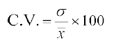
 ,
,
where σ and  , are the standard deviation and mean of the data.
15.6.1 Comparison of two frequency distributions with same mean
Let and
and and σ1 be the mean and standard deviation of the first distribution, and and σ2 be the mean and standard deviation of the second distribution.
Then C.V. (1st distribution) = 
and C.V. (2nd distribution) = 
Given
 = = (say)
Therefore C.V. (1st distribution) = ... (1)
and C.V. (2nd distribution) = ... (2)
It is clear from (1) and (2) that the two C.Vs. can be compared on the basis of values of  and
and only.
only.
Thus, we say that for two series with equal means, the series with greater standard deviation (or variance) is called more variable or dispersed than the other. Also, the series with lesser value of standard deviation (or variance) is said to be more consistent than the other.
Let us now take following examples:
Example 13 Two plants A and B of a factory show following results about the number of workers and the wages paid to them.
A B
No. of workers 5000 6000
Average monthly wages Rs 2500 Rs 2500
Variance of distribution 81 100
of wages
In which plant, A or B is there greater variability in individual wages?
Solution The variance of the distribution of wages in plant A ( ) = 81
Therefore, standard deviation of the distribution of wages in plant A () = 9
Also, the variance of the distribution of wages in plant B ( ) = 100
Therefore, standard deviation of the distribution of wages in plant B ( ) = 10
Since the average monthly wages in both the plants is same, i.e., Rs.2500, therefore, the plant with greater standard deviation will have more variability.
Thus, the plant B has greater variability in the individual wages.
Example 14 Coefficient of variation of two distributions are 60 and 70, and their standard deviations are 21 and 16, respectively. What are their arithmetic means.
Solution Given C.V. (1st distribution) = 60, = 21
C.V. (2nd distribution) = 70, = 16
Let and
and  and be the means of 1st and 2nd distribution, respectively. Then
C.V. (1st distribution) = × 100
× 100
Therefore 60 = 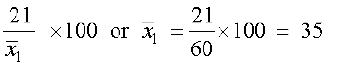
and C.V. (2nd distribution) =  ×100
×100
i.e. 70 = 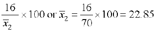
Example 15 The following values are calculated in respect of heights and weights of the students of a section of Class XI :
Height Weight
Mean 162.6 cm 52.36 kg
Variance 127.69 cm2 23.1361 kg2
Can we say that the weights show greater variation than the heights?
Solution To compare the variability, we have to calculate their coefficients of variation.
Given Variance of height = 127.69cm2
Therefore Standard deviation of height = = 11.3 cm
Also Variance of weight = 23.1361 kg2
Therefore Standard deviation of weight = = 4.81 kg
Now, the coefficient of variations (C.V.) are given by
(C.V.) in heights =
= = 6.95
and (C.V.) in weights =  = 9.18
Clearly C.V. in weights is greater than the C.V. in heights
Therefore, we can say that weights show more variability than heights.
Exercise15.3
1. From the data given below state which group is more variable, A or B?
| Marks | 10-20 | 20-30 | 30-40 | 40-50 | 50-60 | 60-70 | 70-80 |
| Group | 9 | 17 | 32 | 33 | 40 | 10 | 9 |
| Group B | 10 | 20 | 30 | 25 | 43 | 15 | 7 |
2. From the prices of shares X and Y below, find out which is more stable in value:
| X | 35 | 54 | 52 | 53 | 56 | 58 | 52 | 50 | 51 | 49 |
| Y | 108 | 107 | 105 | 105 | 106 | 107 | 104 | 103 | 104 | 101 |
3. An analysis of monthly wages paid to workers in two firms A and B, belonging to the same industry, gives the following results:
Firm A Firm B
No. of wage earners 586 648
Mean of monthly wages Rs 5253 Rs 5253
Variance of the distribution 100 121
of wages
(i) Which firm A or B pays larger amount as monthly wages?
(ii) Which firm, A or B, shows greater variability in individual wages?
4. The following is the record of goals scored by team A in a football session:
| No. of goals scored | 0 | 1 | 2 | 3 | 4 |
| No. of matches | 1 | 9 | 7 | 5 | 3 |
For the team B, mean number of goals scored per match was 2 with a standard deviation 1.25 goals. Find which team may be considered more consistent?
5. The sum and sum of squares corresponding to length x (in cm) and weight y
(in gm) of 50 plant products are given below:
 ,
,  ,
, 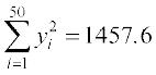 ,
,
Which is more varying, the length or weight?
Miscellaneous Examples
Example 16 The variance of 20 observations is 5. If each observation is multiplied by 2, find the new variance of the resulting observations.
Solution Let the observations be x1, x2, ..., x20 and be their mean. Given that variance = 5 and n = 20. We know that
Variance  , i.e.,
or  = 100 ... (1)
If each observation is multiplied by 2, and the new resulting observations are yi , then
yi = 2xi i.e., xi = 
Therefore 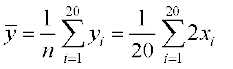 =
= =
=
i.e. = 2 or = 
Substituting the values of xi and in (1), we get
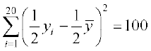 , i.e.,
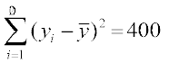 ,
,
Thus the variance of new observations =
Note The reader may note that if each observation is multiplied by a constant k, the variance of the resulting observations becomes k2 times the original variance.
Example17 The mean of 5 observations is 4.4 and their variance is 8.24. If three of the observations are 1, 2 and 6, find the other two observations.
Solution Let the other two observations be x and y.
Therefore, the series is 1, 2, 6, x, y.
Now Mean  = 4.4 =
or 22 = 9 + x + y
Therefore x + y = 13 ... (1)
Alsovariance=8.24 =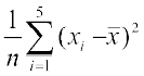
i.e. 8.24 = 
or 41.20 = 11.56 + 5.76 + 2.56 + x2 + y2 –8.8 × 13 + 38.72
Therefore x2 + y2 = 97 ... (2)
But from (1), we have
x2 + y2 + 2xy = 169 ... (3)
From (2) and (3), we have
2xy = 72 ... (4)
Subtracting (4) from (2), we get
x2 + y2 – 2xy = 97 – 72 i.e. (x – y)2 = 25
or x – y =  5 ... (5)
So, from (1) and (5), we get
x = 9, y = 4 when x – y = 5
or x = 4, y = 9 when x – y = – 5
Thus, the remaining observations are 4 and 9.
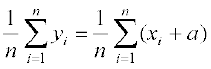
Example 18 If each of the observation x1, x2, ...,xn is increased by ‘a’, where a is a negative or positive number, show that the variance remains unchanged.
Solution Let be the mean of x1, x2, ...,xn . Then the variance is given by
 =
= =
=
If ‘a is added to each observation, the new observations will be
yi = xi + a ... (1)
Let the mean of the new observations be  . Then
=
= 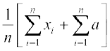
= 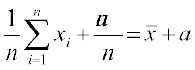
 = + a
= + a
i.e. =  + a ... (2)
Thus, the variance of the new observations
=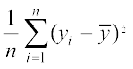 =
= 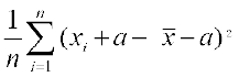 [Using (1) and (2)]
=  =
=  =
=
Thus, the variance of the new observations is same as that of the original observations.
Note We may note that adding (or subtracting) a positive number to (or from) each observation of a group does not affect the variance.
Example 19 The mean and standard deviation of 100 observations were calculated as 40 and 5.1, respectively by a student who took by mistake 50 instead of 40 for one observation. What are the correct mean and standard deviation?
Solution Given that number of observations (n) = 100
Incorrect mean ( ) = 40,
Incorrect standard deviation (σ) = 5.1
We know that 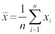
i.e. 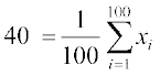 or
or
 = 4000
i.e. Incorrect sum of observations = 4000
Thus the correct sum of observations = Incorrect sum – 50 + 40
= 4000 – 50 + 40 = 3990
Hence Correct mean =  = 39.9
Also Standard deviation = 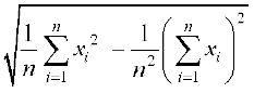
= 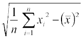
i.e. 5.1= 
or 26.01 =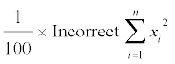
 – 1600
Therefore Incorrect= 100 (26.01 + 1600) = 162601
Now Correct  = Incorrect – (50)2 + (40)2
= 162601 – 2500 + 1600 = 161701
Therefore Correct standard deviation
=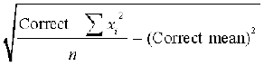
= 
=  =
=  = = 5
= = 5
Miscellaneous Exercise On Chapter 15
1. The mean and variance of eight observations are 9 and 9.25, respectively. If six of the observations are 6, 7, 10, 12, 12 and 13, find the remaining two observations.
2. The mean and variance of 7 observations are 8 and 16, respectively. If five of the observations are 2, 4, 10, 12, 14. Find the remaining two observations.
3. The mean and standard deviation of six observations are 8 and 4, respectively. If each observation is multiplied by 3, find the new mean and new standard deviation of the resulting observations.
4. Given that is the mean and σ2 is the variance of n observations x1, x2, ...,xn. Prove that the mean and variance of the observations ax1, ax2, ax3, ...., axn are a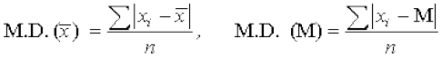 and a2 σ2, respectively, (a ≠ 0).
5. The mean and standard deviation of 20 observations are found to be 10 and 2, respectively. On rechecking, it was found that an observation 8 was incorrect. Calculate the correct mean and standard deviation in each of the following cases:
(i) If wrong item is omitted. (ii) If it is replaced by 12.
6. The mean and standard deviation of marks obtained by 50 students of a class in three subjects, Mathematics, Physics and Chemistry are given below:
Subject Mathematics Physics Chemistry
Mean 42 32 40.9
Standard 12 15 20
deviation
Which of the three subjects shows the highest variability in marks and which shows the lowest?
7. The mean and standard deviation of a group of 100 observations were found to be 20 and 3, respectively. Later on it was found that three observations were incorrect, which were recorded as 21, 21 and 18. Find the mean and standard deviation if the incorrect observations are omitted.
Summary
- Measures of dispersion Range, Quartile deviation, mean deviation, variance, standard deviation are measures of dispersion.
Range = Maximum Value – Minimum Value
- Mean deviation for ungrouped data

- Mean deviation for grouped data

- Variance and standard deviation for ungrouped data
 ,
, 
- Variance and standard deviation of a discrete frequency distribution
- Variance and standard deviation of a continuous frequency distribution
- Shortcut method to find variance and standard deviation.
 ,
,  ,
,
where 
- Coefficient of variation (C.V.)
For series with equal means, the series with lesser standard deviation is more consistent or less scattered.
Historical Note
‘Statistics’ is derived from the Latin word ‘status’ which means a political state. This suggests that statistics is as old as human civilisation. In the year 3050 B.C., perhaps the first census was held in Egypt. In India also, about 2000 years ago, we had an efficient system of collecting administrative statistics, particularly, during the regime of Chandra Gupta Maurya (324-300 B.C.). The system of collecting data related to births and deaths is mentioned in Kautilya’s Arthshastra (around 300 B.C.) A detailed account of administrative surveys conducted during Akbar’s regime is given in Ain-I-Akbari written by Abul Fazl.
Captain John Graunt of London (1620-1674) is known as father of vital statistics due to his studies on statistics of births and deaths. Jacob Bernoulli (1654-1705) stated the Law of Large numbers in his book “Ars Conjectandi’, published in 1713.
The theoretical development of statistics came during the mid seventeenth century and continued after that with the introduction of theory of games and chance (i.e., probability). Francis Galton (1822-1921), an Englishman, pioneered the use of statistical methods, in the field of Biometry. Karl Pearson (1857-1936) contributed a lot to the development of statistical studies with his discovery of Chi square test and foundation of statistical laboratory in England (1911). Sir Ronald A. Fisher (1890-1962), known as the Father of modern statistics, applied it to various diversified fields such as Genetics, Biometry, Education, Agriculture, etc.