Table of Contents
Chapter One
Units and Measurement

1.1 Introduction
1.2 The international system of units
1.3 Significant figures
1.4 Dimensions of physical quantities
1.5 Dimensional formulae and dimensional equations
1.6 Dimensional analysis and its applications
Summary
Exercises
Additional exercises
1.1 Introduction
Measurement of any physical quantity involves comparison with a certain basic, arbitrarily chosen, internationally accepted reference standard called unit. The result of a measurement of a physical quantity is expressed by a number (or numerical measure) accompanied by a unit. Although the number of physical quantities appears to be very large, we need only a limited number of units for expressing all the physical quantities, since they are inter-related with one another. The units for the fundamental or base quantities are called fundamental or base units. The units of all other physical quantities can be expressed as combinations of the base units. Such units obtained for the derived quantities are called derived units. A complete set of these units, both the base units and derived units, is known as the system of units.
1.2 The International System of Units
In earlier time scientists of different countries were using different systems of units for measurement. Three such systems, the CGS, the FPS (or British) system and the MKS system were in use extensively till recently.
The base units for length, mass and time in these systems were as follows :
• In CGS system they were centimetre, gram and second respectively.
• In FPS system they were foot, pound and second respectively.
• In MKS system they were metre, kilogram and second respectively.
The system of units which is at present internationally accepted for measurement is the Système Internationale
d’ Unites (French for International System of Units), abbreviated as SI. The SI, with standard scheme of symbols, units and abbreviations, developed by the Bureau International des Poids et measures (The International Bureau of weights and measures, BIPM) in 1971 were recently revised by the General Conference on weights and measures in November 2018. The scheme is now for international usage in scientific, technical, industrial and commercial work. Because SI units used decimal system, conversions within the system are quite simple and convenient. We shall follow the SI units in this book.
In SI, there are seven base units as given in Table 2.1. Besides the seven base units, there are two more units that are defined for (a) plane angle dθ as the ratio of length of arc ds to the radius r and (b) solid angle dΩ as the ratio of the intercepted area dA of the spherical surface, described about the apex O as the centre, to the square of its radius r, as shown in Fig. 2.1(a) and (b) respectively. The unit for plane angle is radian with the symbol rad and the unit for the solid angle is steradian with the symbol sr. Both these are dimensionless quantities.
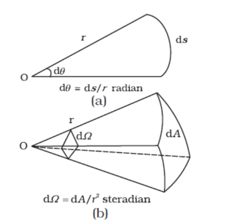
Fig. 1.1 Description of (a) plane angle dθ and (b) solid angle
Table 1.1 SI Base Quantities and Units*
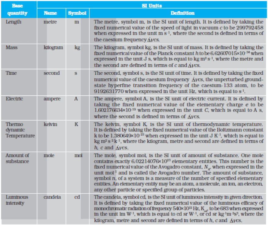
* The values mentioned here need not be remembered or asked in a test. They are given here only to indicate the extent of accuracy to which they are measured. With progress in technology, the measuring techniques get improved leading to measurements with greater precision. The definitions of base units are revised to keep up with this progress.
Table 1.2 Some units retained for general use (Though outside SI)
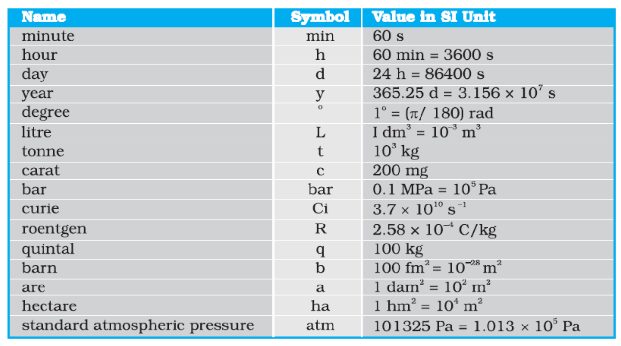
Note that when mole is used, the elementary entities must be specified. These entities may be atoms, molecules, ions, electrons, other particles or specified groups of such particles.
We employ units for some physical quantities that can be derived from the seven base units (Appendix A 6). Some derived units in terms of the SI base units are given in (Appendix A 6.1). Some SI derived units are given special names (Appendix A 6.2 ) and some derived SI units make use of these units with special names and the seven base units (Appendix A 6.3). These are given in Appendix A 6.2 and A 6.3 for your ready reference. Other units retained for general use are given in Table 2.2.
Common SI prefixes and symbols for multiples and sub-multiples are given in Appendix A2. General guidelines for using symbols for physical quantities, chemical elements and nuclides are given in Appendix A7 and those for SI units and some other units are given in Appendix A8 for your guidance and ready reference.
1.3 Significant figures
As discussed above, every measurement involves errors. Thus, the result of measurement should be reported in a way that indicates the precision of measurement. Normally, the reported result of measurement is a number that includes all digits in the number that are known reliably plus the first digit that is uncertain. The reliable digits plus the first uncertain digit are known as significant digits or significant figures. If we say the period of oscillation of a simple pendulum is 1.62 s, the digits 1 and 6 are reliable and certain, while the digit 2 is uncertain. Thus, the measured value has three significant figures. The length of an object reported after measurement to be 287.5 cm has four significant figures, the digits 2, 8, 7 are certain while the digit 5 is uncertain. Clearly, reporting the result of measurement that includes more digits than the significant digits is superfluous and also misleading since it would give a wrong idea about the precision of measurement.
The rules for determining the number of significant figures can be understood from the following examples. Significant figures indicate, as already mentioned, the precision of measurement which depends on the least count of the measuring instrument. A choice of change of different units does not change the number of significant digits or figures in a measurement. This important remark makes most of the following observations clear:
(1) For example, the length 2.308 cm has four significant figures. But in different units, the same value can be written as 0.02308 m or 23.08 mm or 23080 µm.
All these numbers have the same number of significant figures (digits 2, 3, 0, 8), namely four. This shows that the location of decimal point is of no consequence in determining the number of significant figures.
The example gives the following rules :
• All the non-zero digits are significant.
• All the zeros between two non-zero digits are significant, no matter where the decimal point is, if at all.
• If the number is less than 1, the zero(s) on the right of decimal point but to the left of the first non-zero digit are not significant. [In 0.00 2308, the underlined zeroes are not significant].
• The terminal or trailing zero(s) in a number without a decimal point are not significant.
[Thus 123 m = 12300 cm = 123000 mm has three significant figures, the trailing zero(s) being not significant.] However, you can also see the next observation.
• The trailing zero(s) in a number with a decimal point are significant.
[The numbers 3.500 or 0.06900 have four significant figures each.]
(2) There can be some confusion regarding the trailing zero(s). Suppose a length is reported to be 4.700 m. It is evident that the zeroes here are meant to convey the precision of measurement and are, therefore, significant. [If these were not, it would be superfluous to write them explicitly, the reported measurement would have been simply 4.7 m]. Now suppose we change units, then
4.700 m = 470.0 cm = 4700 mm = 0.004700 km
Since the last number has trailing zero(s) in a number with no decimal, we would conclude erroneously from observation (1) above that the number has two significant figures, while in fact, it has four significant figures and a mere change of units cannot change the number of significant figures.
(3) To remove such ambiguities in determining the number of significant figures, the best way is to report every measurement in scientific notation (in the power of 10). In this notation, every number is expressed as a × 10b, where a is a number between 1 and 10, and b is any positive or negative exponent (or power) of 10. In order to get an approximate idea of the number, we may round off the number a to 1 (for a  5) and to 10 (for 5<a
 10). Then the number can be expressed approximately as 10b in which the exponent (or power) b of 10 is called order of magnitude of the physical quantity. When only an estimate is required, the quantity is of the order of 10b. For example, the diameter of the earth (1.28×10⁷m) is of the order of 107m with the order of magnitude 7. The diameter of hydrogen atom (1.06 ×10⁻¹⁰m) is of the order of 10–10m, with the order of magnitude
–10. Thus, the diameter of the earth is 17 orders of magnitude larger than the hydrogen atom.
It is often customary to write the decimal after the first digit. Now the confusion mentioned in (a) above disappears :
4.700 m = 4.700 × 102 cm
= 4.700 × 103 mm = 4.700 × 10⁻³ km
The power of 10 is irrelevant to the determination of significant figures. However, all zeroes appearing in the base number in the scientific notation are significant. Each number in this case has four significant figures.
Thus, in the scientific notation, no confusion arises about the trailing zero(s) in the base number a. They are always significant.
(4) The scientific notation is ideal for reporting measurement. But if this is not adopted, we use the rules adopted in the preceding example :
• For a number greater than 1, without any decimal, the trailing zero(s) are not significant.
• For a number with a decimal, the trailing zero(s) are significant.
(5) The digit 0 conventionally put on the left of a decimal for a number less than 1 (like 0.1250) is never significant. However, the zeroes at the end of such number are significant in a measurement.
(6) The multiplying or dividing factors which are neither rounded numbers nor numbers representing measured values are exact and have infinite number of significant digits. For example in  or s = 2πr, the factor 2 is an exact number and it can be written as 2.0, 2.00 or 2.0000 as required. Similarly, in
  , n is an exact number.
1.3.1 Rules for Arithmetic Operations with Significant Figures
The result of a calculation involving approximate measured values of quantities (i.e. values with limited number of significant figures) must reflect the uncertainties in the original measured values. It cannot be more accurate than the original measured values themselves on which the result is based. In general, the final result should not have more significant figures than the original data from which it was obtained. Thus, if mass of an object is measured to be, say, 4.237 g (four significant figures) and its volume is measured to be 2.51 cm3, then its density, by mere arithmetic division, is 1.68804780876 g/cm3 upto 11 decimal places. It would be clearly absurd and irrelevant to record the calculated value of density to such a precision when the measurements on which the value is based, have much less precision. The following rules for arithmetic operations with significant figures ensure that the final result of a calculation is shown with the precision that is consistent with the precision of the input measured values :
(1) In multiplication or division, the final result should retain as many significant figures as are there in the original number with the least significant figures.
Thus, in the example above, density should be reported to three significant figures.

Similarly, if the speed of light is given as
3 × 10⁸ m s-1 (one significant figure) and one year (1y = 365.25 d) has 3.1557 × 10⁷ s (five significant figures), the light year is 9.47 × 10¹⁵ m (three significant figures).
(2) In addition or subtraction, the final result should retain as many decimal places as are there in the number with the least decimal places.
For example, the sum of the numbers 436.32 g, 227.2 g and 0.301 g by mere arithmetic addition, is 663.821 g. But the least precise measurement (227.2 g) is correct to only one decimal place. The final result should, therefore, be rounded off to 663.8 g.
Similarly, the difference in length can be expressed as :
0.307 m – 0.304 m = 0.003 m = 3 × 10⁻³ m.
Note that we should not use the rule (1) applicable for multiplication and division and write 664 g as the result in the example of addition and 3.00 × 10⁻³ m in the example of subtraction. They do not convey the precision of measurement properly. For addition and subtraction, the rule is in terms of decimal places.
1.3.2 Rounding off the Uncertain Digits
The result of computation with approximate numbers, which contain more than one uncertain digit, should be rounded off. The rules for rounding off numbers to the appropriate significant figures are obvious in most cases. A number 2.746 rounded off to three significant figures is 2.75, while the number 2.743 would be 2.74. The rule by convention is that the preceding digit is raised by 1 if the insignificant digit to be dropped (the underlined digit in this case) is more than 5, and is left unchanged if the latter is less than 5. But what if the number is 2.745 in which the insignificant digit is 5. Here, the convention is that if the preceding digit is even, the insignificant digit is simply dropped and, if it is odd, the preceding digit is raised by 1. Then, the number 2.745 rounded off to three significant figures becomes 2.74. On the other hand, the number 2.735 rounded off to three significant figures becomes 2.74 since the preceding digit is odd.
In any involved or complex multi-step calculation, you should retain, in intermediate steps, one digit more than the significant digits and round off to proper significant figures at the end of the calculation. Similarly, a number known to be within many significant figures, such as in 2.99792458 × 10⁸ m/s for the speed of light in vacuum, is rounded off to an approximate value 3 × 10⁸ m/s , which is often employed in computations. Finally, remember that exact numbers that appear in formulae like 2 π in 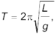 have a large (infinite) number of significant figures. The value of π = 3.1415926.... is known to a large number of significant figures. You may take the value as 3.142 or 3.14 for π, with limited number of significant figures as required in specific
cases.
Example 1.1 Each side of a cube is measured to be 7.203 m. What are the total surface area and the volume of the cube to appropriate significant figures?
Answer The number of significant figures in the measured length is 4. The calculated area and the volume should therefore be rounded off to 4 significant figures.
Surface area of the cube = 6(7.203)2 m2
= 311.299254 m2
= 311.3 m2
Volume of the cube = (7.203)3 m3
= 373.714754 m3
= 373.7 m3
Example 1.2 5.74 g of a substance occupies 1.2 cm3. Express its density by keeping the significant figures in view.
Answer There are 3 significant figures in the measured mass whereas there are only 2 significant figures in the measured volume. Hence the density should be expressed to only 2 significant figures.
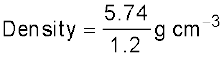
= 4.8 g cm--3 .
1.3.3 Rules for Determining the Uncertainty in the Results of Arithmatic Calculations
The rules for determining the uncertainty or error in the number/measured quantity in arithmetic operations can be understood from the following examples.
(1) If the length and breadth of a thin rectangular sheet are measured, using a metre scale as 16.2 cm and, 10.1 cm respectively, there are three significant figures in each measurement. It means that the length l may be written as
l = 16.2 ± 0.1 cm
= 16.2 cm ± 0.6 %.
Similarly, the breadth b may be written as
b = 10.1 ± 0.1 cm
= 10.1 cm ± 1 %
Then, the error of the product of two (or more) experimental values, using the combination of errors rule, will be
l b = 163.62 cm2 + 1.6%
= 163.62 + 2.6 cm2
This leads us to quote the final result as
l b = 164 + 3 cm2
Here 3 cm2 is the uncertainty or error in the estimation of area of rectangular sheet.
(2) If a set of experimental data is specified to n significant figures, a result obtained by combining the data will also be valid to n significant figures.
However, if data are subtracted, the number of significant figures can be reduced.
For example, 12.9 g – 7.06 g, both specified to three significant figures, cannot properly be evaluated as 5.84 g but only as 5.8 g, as uncertainties in subtraction or addition combine in a different fashion (smallest number of decimal places rather than the number of significant figures in any of the number added or subtracted).
(3) The relative error of a value of number specified to significant figures depends not only on n but also on the number itself.
For example, the accuracy in measurement of mass 1.02 g is ± 0.01 g whereas another measurement 9.89 g is also accurate to ± 0.01 g.
The relative error in 1.02 g is
= (± 0.01/1.02) × 100 %
= ± 1%
Similarly, the relative error in 9.89 g is
= (± 0.01/9.89) × 100 %
= ± 0.1 %
Finally, remember that intermediate results in a multi-step computation should be calculated to one more significant figure in every measurement than the number of digits in the least precise measurement. These should be justified by the data and then the arithmetic operations may be carried out; otherwise rounding errors can build up. For example, the reciprocal of 9.58, calculated (after rounding off) to the same number of significant figures (three) is 0.104, but the reciprocal of 0.104 calculated to three significant figures is 9.62. However, if we had written 1/9.58 = 0.1044 and then taken the reciprocal to three significant figures, we would have retrieved the original value of 9.58.
This example justifies the idea to retain one more extra digit (than the number of digits in the least precise measurement) in intermediate steps of the complex multi-step calculations in order to avoid additional errors in the process of rounding off the numbers.
1.4 Dimensions of physical quantities
The nature of a physical quantity is described by its dimensions. All the physical quantities represented by derived units can be expressed in terms of some combination of seven fundamental or base quantities. We shall call these base quantities as the seven dimensions of the physical world, which are denoted with square brackets [ ]. Thus, length has the dimension [L], mass [M], time [T], electric current [A], thermodynamic temperature [K], luminous intensity [cd], and amount of substance [mol]. The dimensions of a physical quantity are the powers (or exponents) to which the base quantities are raised to represent that quantity. Note that using the square brackets
[ ] round a quantity means that we are dealing with ‘the dimensions of’ the quantity.
In mechanics, all the physical quantities can be written in terms of the dimensions [L], [M] and [T]. For example, the volume occupied by an object is expressed as the product of length, breadth and height, or three lengths. Hence the dimensions of volume are [L] × [L] × [L] = [L]3 = [L3]. As the volume is independent of mass and time, it is said to possess zero dimension in mass [M°], zero dimension in time [T°] and three dimensions in length.
Similarly, force, as the product of mass and acceleration, can be expressed as
Force = mass × acceleration
= mass × (length)/(time)2
The dimensions of force are [M] [L]/[T]2 = [M L T–2]. Thus, the force has one dimension in mass, one dimension in length, and –2 dimensions in time. The dimensions in all other base quantities are zero.
Note that in this type of representation, the magnitudes are not considered. It is the quality of the type of the physical quantity that enters. Thus, a change in velocity, initial velocity, average velocity, final velocity, and speed are all equivalent in this context. Since all these quantities can be expressed as length/time, their dimensions are [L]/[T] or [L T–1].
1.5 Dimensional formulae and dimensional Equations
The expression which shows how and which of the base quantities represent the dimensions of a physical quantity is called the dimensional formula of the given physical quantity. For example, the dimensional formula of the volume is [M° L3 T°], and that of speed or velocity is
[M° L T-1]. Similarly, [M° L T–2] is the dimensional formula of acceleration and [M L–3 T°] that of mass density.
An equation obtained by equating a physical quantity with its dimensional formula is called the dimensional equation of the physical quantity. Thus, the dimensional equations are the equations, which represent the dimensions of a physical quantity in terms of the base quantities. For example, the dimensional equations of volume [V], speed [v], force [F] and mass density [ρ] may be expressed as
[V] = [M0 L3 T0]
[v] = [M0 L T–1]
[F] = [M L T–2]
[ρ] = [M L–3 T0]
The dimensional equation can be obtained from the equation representing the relations between the physical quantities. The dimensional formulae of a large number and wide variety of physical quantities, derived from the equations representing the relationships among other physical quantities and expressed in terms of base quantities are given in Appendix 9 for your guidance and ready reference.
1.6 Dimensional analysis and its applications
The recognition of concepts of dimensions, which guide the description of physical behaviour is of basic importance as only those physical quantities can be added or subtracted which have the same dimensions. A thorough understanding of dimensional analysis helps us in deducing certain relations among different physical quantities and checking the derivation, accuracy and dimensional consistency or homogeneity of various mathematical expressions. When magnitudes of two or more physical quantities are multiplied, their units should be treated in the same manner as ordinary algebraic symbols. We can cancel identical units in the numerator and denominator. The same is true for dimensions of a physical quantity. Similarly, physical quantities represented by symbols on both sides of a mathematical equation must have the same dimensions.
1.6.1 Checking the Dimensional Consistency of Equations
The magnitudes of physical quantities may be added together or subtracted from one another only if they have the same dimensions. In other words, we can add or subtract similar physical quantities. Thus, velocity cannot be added to force, or an electric current cannot be subtracted from the thermodynamic temperature. This simple principle called the principle of homogeneity of dimensions in an equation is extremely useful in checking the correctness of an equation. If the dimensions of all the terms are not same, the equation is wrong. Hence, if we derive an expression for the length (or distance) of an object, regardless of the symbols appearing in the original mathematical relation, when all the individual dimensions are simplified, the remaining dimension must be that of length. Similarly, if we derive an equation of speed, the dimensions on both the sides of equation, when simplified, must be of length/time, or [L T–1].
Dimensions are customarily used as a preliminary test of the consistency of an equation, when there is some doubt about the correctness of the equation. However, the dimensional consistency does not guarantee correct equations. It is uncertain to the extent of dimensionless quantities or functions. The arguments of special functions, such as the trigonometric, logarithmic and exponential functions must be dimensionless. A pure number, ratio of similar physical quantities, such as angle as the ratio (length/length), refractive index as the ratio (speed of light in vacuum/speed of light in medium) etc., has no dimensions.
Now we can test the dimensional consistency or homogeneity of the equation
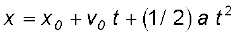
for the distance x travelled by a particle or body in time t which starts from the position x0 with an initial velocity v0 at time t = 0 and has uniform acceleration a along the direction of motion.
The dimensions of each term may be written as
[x] = [L]
[x0 ] = [L]
[v0 t] = [L T–1] [T]
= [L]
[(1/2) a t2] = [L T–2] [T2]
= [L]
As each term on the right hand side of this equation has the same dimension, namely that of length, which is same as the dimension of left hand side of the equation, hence this equation is a dimensionally correct equation.
It may be noted that a test of consistency of dimensions tells us no more and no less than a test of consistency of units, but has the advantage that we need not commit ourselves to a particular choice of units, and we need not worry about conversions among multiples and sub-multiples of the units. It may be borne in mind that if an equation fails this consistency test, it is proved wrong, but if it passes, it is not proved right. Thus, a dimensionally correct equation need not be actually an exact (correct) equation, but a dimensionally wrong (incorrect) or inconsistent equation must be wrong.
Example 1.3 Let us consider an equation
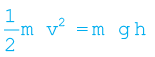
where m is the mass of the body, v its velocity, g is the acceleration due to gravity and h is the height. Check whether this equation is dimensionally correct.
Answer The dimensions of LHS are
[M] [L T–1 ]2 = [M] [ L2 T–2]
= [M L2 T–2]
The dimensions of RHS are
[M][L T–2] [L] = [M][L2 T–2]
= [M L2 T–2]
The dimensions of LHS and RHS are the same and hence the equation is dimensionally correct.
Example 1.4 The SI unit of energy is
J = kg m2 s–2; that of speed v is m s–1 and of acceleration a is m s–2. Which of the formulae for kinetic energy (K) given below can you rule out on the basis of dimensional arguments (m stands for the mass of the body) :
(a) K = m2 v3
(b) K = (1/2)mv2
(c) K = ma
(d) K = (3/16)mv2
(e) K = (1/2)mv2 + ma
Answer Every correct formula or equation must have the same dimensions on both sides of the equation. Also, only quantities with the same physical dimensions can be added or subtracted. The dimensions of the quantity on the right side are [M2 L3 T–3]