Table of Contents
Chapter Thour
Laws of Motion

4.1 Introduction
4.2 Aristotle’s fallacy
4.3 The law of inertia
4.4 Newton’s first law of motion
4.5 Newton’s second law of motion
4.6 Newton’s third law of motion
4.7 Conservation of momentum
4.8 Equilibrium of a particle
4.9 Common forces in mechanics
4.10 Circular motion
4.11 Solving problems in mechanics
Summary
Points to ponder
Exercises
Additional exercises
4.1 INTRODUCTION
In the preceding Chapter, our concern was to describe the motion of a particle in space quantitatively. We saw that uniform motion needs the concept of velocity alone whereas non-uniform motion requires the concept of acceleration in addition. So far, we have not asked the question as to what governs the motion of bodies. In this chapter, we turn to this basic question.
Let us first guess the answer based on our common experience. To move a football at rest, someone must kick it. To throw a stone upwards, one has to give it an upward push. A breeze causes the branches of a tree to swing; a strong wind can even move heavy objects. A boat moves in a flowing river without anyone rowing it. Clearly, some external agency is needed to provide force to move a body from rest. Likewise, an external force is needed also to retard or stop motion. You can stop a ball rolling down an inclined plane by applying a force against the direction of its motion.
In these examples, the external agency of force (hands, wind, stream, etc) is in contact with the object. This is not always necessary. A stone released from the top of a building accelerates downward due to the gravitational pull of the earth. A bar magnet can attract an iron nail from a distance. This shows that external agencies (e.g. gravitational and magnetic forces ) can exert force on a body even from a distance.
In short, a force is required to put a stationary body in motion or stop a moving body, and some external agency is needed to provide this force. The external agency may or may not be in contact with the body.
So far so good. But what if a body is moving uniformly (e.g. a skater moving straight with constant speed on a horizontal ice slab) ? Is an external force required to keep a body in uniform motion?
4.2 Aristotle’s fallacy
The question posed above appears to be simple. However, it took ages to answer it. Indeed, the correct answer to this question given by Galileo in the seventeenth century was the foundation of Newtonian mechanics, which signalled the birth of modern science.
The Greek thinker, Aristotle (384 B.C– 322 B.C.), held the view that if a body is moving, something external is required to keep it moving. According to this view, for example, an arrow shot from a bow keeps flying since the air behind the arrow keeps pushing it. The view was part of an elaborate framework of ideas developed by Aristotle on the motion of bodies in the universe. Most of the Aristotelian ideas on motion are now known to be wrong and need not concern us. For our purpose here, the Aristotelian law of motion may be phrased thus: An external force is required to keep a body in motion.
Aristotelian law of motion is flawed, as we shall see. However, it is a natural view that anyone would hold from common experience. Even a small child playing with a simple (non-electric) toy-car on a floor knows intuitively that it needs to constantly drag the string attached to the toy-car with some force to keep it going. If it releases the string, it comes to rest. This experience is common to most terrestrial motion. External forces seem to be needed to keep bodies in motion. Left to themselves, all bodies eventually come to rest.
What is the flaw in Aristotle’s argument? The answer is: a moving toy car comes to rest because the external force of friction on the car by the floor opposes its motion. To counter this force, the child has to apply an external force on the car in the direction of motion. When the car is in uniform motion, there is no net external force acting on it: the force by the child cancels the force ( friction) by the floor. The corollary is: if there were no friction, the child would not be required to apply any force to keep the toy car in uniform motion.
The opposing forces such as friction (solids) and viscous forces (for fluids) are always present in the natural world. This explains why forces by external agencies are necessary to overcome the frictional forces to keep bodies in uniform motion. Now we understand where Aristotle went wrong. He coded this practical experience in the form of a basic argument. To get at the true law of nature for forces and motion, one has to imagine a world in which uniform motion is possible with no frictional forces opposing. This is what Galileo did.
4.3 The law of inertia
Galileo studied motion of objects on an inclined plane. Objects (i) moving down an inclined plane accelerate, while those (ii) moving up retard.
(iii) Motion on a horizontal plane is an intermediate situation. Galileo concluded that an object moving on a frictionless horizontal plane must neither have acceleration nor retardation, i.e. it should move with constant velocity (Fig. 4.1(a)).

(i) (ii) (iii)
Fig. 4.1(a)
Another experiment by Galileo leading to the same conclusion involves a double inclined plane. A ball released from rest on one of the planes rolls down and climbs up the other. If the planes are smooth, the final height of the ball is nearly the same as the initial height (a little less but never greater). In the ideal situation, when friction is absent, the final height of the ball is the same as its initial height.
If the slope of the second plane is decreased and the experiment repeated, the ball will still reach the same height, but in doing so, it will travel a longer distance. In the limiting case, when the slope of the second plane is zero (i.e. is a horizontal) the ball travels an infinite distance. In other words, its motion never ceases. This is, of course, an idealised situation (Fig. 4.1(b)).
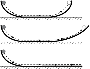
Fig. 4.1(b) The law of inertia was inferred by Galileo from observations of motion of a ball on a double inclined plane.
In practice, the ball does come to a stop after moving a finite distance on the horizontal plane, because of the opposing force of friction which can never be totally eliminated. However, if there were no friction, the ball would continue to move with a constant velocity on the horizontal plane.
Galileo thus, arrived at a new insight on motion that had eluded Aristotle and those who followed him. The state of rest and the state of uniform linear motion (motion with constant velocity) are equivalent. In both cases, there is no net force acting on the body. It is incorrect to assume that a net force is needed to keep a body in uniform motion. To maintain a body in uniform motion, we need to apply an external force to ecounter the frictional force, so that the two forces sum up to zero net external force.
To summarise, if the net external force is zero, a body at rest continues to remain at rest and a body in motion continues to move with a uniform velocity. This property of the body is called inertia. Inertia means ‘resistance to change’. A body does not change its state of rest or uniform motion, unless an external force compels it to change that state.
Ideas on Motion in Ancient Indian Science
Ancient Indian thinkers had arrived at an elaborate system of ideas on motion. Force, the cause of motion, was thought to be of different kinds : force due to continuous pressure (nodan), as the force of wind on a sailing vessel; impact (abhighat), as when a potter’s rod strikes the wheel; persistent tendency (sanskara) to move in a straight line(vega) or restoration of shape in an elastic body; transmitted force by a string, rod, etc. The notion of (vega) in the Vaisesika theory of motion perhaps comes closest to the concept of inertia. Vega, the tendency to move in a straight line, was thought to be opposed by contact with objects including atmosphere, a parallel to the ideas of friction and air resistance. It was correctly summarised that the different kinds of motion (translational, rotational and vibrational) of an extended body arise from only the translational motion of its constituent particles. A falling leaf in the wind may have downward motion as a whole (patan) and also rotational and vibrational motion (bhraman, spandan), but each particle of the leaf at an instant only has a definite (small) displacement. There was considerable focus in Indian thought on measurement of motion and units of length and time. It was known that the position of a particle in space can be indicated by distance measured along three axes. Bhaskara (1150 A.D.) had introduced the concept of ‘instantaneous motion’ (tatkaliki gati), which anticipated the modern notion of instantaneous velocity using Differential Calculus. The difference between a wave and a current (of water) was clearly understood; a current is a motion of particles of water under gravity and fluidity while a wave results from the transmission of vibrations of water particles.
4.4 Newton’s First Law of motion
Galileo’s simple, but revolutionary ideas dethroned Aristotelian mechanics. A new mechanics had to be developed. This task was accomplished almost single-handedly by Isaac Newton, one of the greatest scientists of all times.
Newton built on Galileo’s ideas and laid the foundation of mechanics in terms of three laws of motion that go by his name. Galileo’s law of inertia was his starting point which he formulated as the first law of motion:
Every body continues to be in its state of rest or of uniform motion in a straight line unless compelled by some external force to act otherwise.
The state of rest or uniform linear motion both imply zero acceleration. The first law of motion can, therefore, be simply expressed as:
If the net external force on a body is zero, its acceleration is zero. Acceleration can be non zero only if there is a net external force on the body.
Two kinds of situations are encountered in the application of this law in practice. In some examples, we know that the net external force on the object is zero. In that case we can conclude that the acceleration of the object is zero. For example, a spaceship out in interstellar space, far from all other objects and with all its rockets turned off, has no net external force acting on it. Its acceleration, according to the first law, must be zero. If it is in motion, it must continue to move with a uniform velocity.
Galileo Galilei (1564 - 1642)
Galileo Galilei, born in Pisa, Italy in 1564 was a key figure in the scientific revolution in Europe about four centuries ago. Galileo proposed the concept of acceleration. From experiments on motion of bodies on inclined planes or falling freely, he contradicted the Aristotelian notion that a force was required to keep a body in motion, and that heavier bodies fall faster than lighter bodies under gravity. He thus arrived at the law of inertia that was the starting point of the subsequent epochal work of Isaac Newton.
Galileo’s discoveries in astronomy were equally revolutionary. In 1609, he designed his own telescope (invented earlier in Holland) and used it to make a number of startling observations : mountains and depressions on the surface of the moon; dark spots on the sun; the moons of Jupiter and the phases of Venus. He concluded that the Milky Way derived its luminosity because of a large number of stars not visible to the naked eye. In his masterpiece of scientific reasoning : Dialogue on the Two Chief World Systems, Galileo advocated the heliocentric theory of the solar system proposed by Copernicus, which eventually got universal acceptance.
With Galileo came a turning point in the very method of scientific inquiry. Science was no longer merely observations of nature and inferences from them. Science meant devising and doing experiments to verify or refute theories. Science meant measurement of quantities and a search for mathematical relations between them. Not undeservedly, many regard Galileo as the father of modern science.
More often, however, we do not know all the forces to begin with. In that case, if we know that an object is unaccelerated (i.e. it is either at rest or in uniform linear motion), we can infer from the first law that the net external force on the object must be zero. Gravity is everywhere. For terrestrial phenomena, in particular, every object experiences gravitational force due to the earth. Also objects in motion generally experience friction, viscous drag, etc. If then, on earth, an object is at rest or in uniform linear motion, it is not because there are no forces acting on it, but because the various external forces cancel out i.e. add up to zero net external force.
Consider a book at rest on a horizontal surface Fig. (4.2(a)). It is subject to two external forces : the force due to gravity (i.e. its weight W) acting downward and the upward force on the book by the table, the normal force R . R is a self-adjusting force. This is an example of the kind of situation mentioned above. The forces are not quite known fully but the state of motion is known. We observe the book to be at rest. Therefore, we conclude from the first law that the magnitude of R equals that of W. A statement often encountered is : “Since W = R, forces cancel and, therefore, the book is at rest”. This is incorrect reasoning. The correct statement is : “Since the book is observed to be at rest, the net external force on it must be zero, according to the first law. This implies that the normal force R must be equal and opposite to the weight W ”.
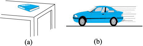
Fig. 4.2 (a) a book at rest on the table, and (b) a car moving with uniform velocity. The net force is zero in each case.
Consider the motion of a car starting from rest, picking up speed and then moving on a smooth straight road with uniform speed (Fig. (4.2(b)). When the car is stationary, there is no net force acting on it. During pick-up, it accelerates. This must happen due to a net external force. Note, it has to be an external force. The acceleration of the car cannot be accounted for by any internal force. This might sound surprising, but it is true. The only conceivable external force along the road is the force of friction. It is the frictional force that accelerates the car as a whole. (You will learn about friction in section 4.9). When the car moves with constant velocity, there is no net external force.
The property of inertia contained in the First law is evident in many situations. Suppose we are standing in a stationary bus and the driver starts the bus suddenly. We get thrown backward with a jerk. Why ? Our feet are in touch with the floor. If there were no friction, we would remain where we were, while the floor of the bus would simply slip forward under our feet and the back of the bus would hit us. However, fortunately, there is some friction between the feet and the floor. If the start is not too sudden, i.e. if the acceleration is moderate, the frictional force would be enough to accelerate our feet along with the bus. But our body is not strictly a rigid body. It is deformable, i.e. it allows some relative displacement between different parts. What this means is that while our feet go with the bus, the rest of the body remains where it is due to inertia. Relative to the bus, therefore, we are thrown backward. As soon as that happens, however, the muscular forces on the rest of the body (by the feet) come into play to move the body along with the bus. A similar thing happens when the bus suddenly stops. Our feet stop due to the friction which does not allow relative motion between the feet and the floor of the bus. But the rest of the body continues to move forward due to inertia. We are thrown forward. The restoring muscular forces again come into play and bring the body to rest.
Example 4.1 An astronaut accidentally gets separated out of his small spaceship accelerating in inter stellar space at a constant rate of 100 m s–2. What is the acceleration of the astronaut the instant after he is outside the spaceship ? (Assume that there are no nearby stars to exert gravitational force on him.)
Answer Since there are no nearby stars to exert gravitational force on him and the small spaceship exerts negligible gravitational attraction on him, the net force acting on the astronaut, once he is out of the spaceship, is zero. By the first law of motion the acceleration of the astronaut is zero.
4.5 Newton’s Second Law of motion
The first law refers to the simple case when the net external force on a body is zero. The second law of motion refers to the general situation when there is a net external force acting on the body. It relates the net external force to the acceleration of the body.
Momentum
Momentum of a body is defined to be the product of its mass m and velocity v, and is denoted
by p:
p = m v (5.1)
Momentum is clearly a vector quantity. The following common experiences indicate the importance of this quantity for considering the effect of force on motion.
• Suppose a light-weight vehicle (say a small car) and a heavy weight vehicle (say a loaded truck) are parked on a horizontal road. We all know that a much greater force is needed to push the truck than the car to bring them to the same speed in same time. Similarly, a greater opposing force is needed to stop a heavy body than a light body in the same time, if they are moving with the same speed.
• If two stones, one light and the other heavy, are dropped from the top of a building, a person on the ground will find it easier to catch the light stone than the heavy stone. The mass of a body is thus an important parameter that determines the effect of force on its motion.
• Speed is another important parameter to consider. A bullet fired by a gun can easily pierce human tissue before it stops, resulting in casualty. The same bullet fired with moderate speed will not cause much damage. Thus for a given mass, the greater the speed, the greater is the opposing force needed to stop the body in a certain time. Taken together, the product of mass and velocity, that is momentum, is evidently a relevant variable of motion. The greater the change in the momentum in a given time, the greater is the force that needs to be applied.
• A seasoned cricketer catches a cricket ball coming in with great speed far more easily than a novice, who can hurt his hands in the act. One reason is that the cricketer allows a longer time for his hands to stop the ball. As you may have noticed, he draws in the hands backward in the act of catching the ball (Fig. 4.3). The novice, on the other hand, keeps his hands fixed and tries to catch the ball almost instantly. He needs to provide a much greater force to stop the ball instantly, and this hurts. The conclusion is clear: force not only depends on the change in momentum, but also on how fast the change is brought about. The same change in momentum brought about in a shorter time needs a greater applied force. In short, the greater the rate of change of momentum, the greater is the force.
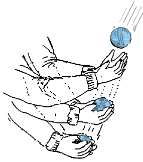
Fig. 4.3 Force not only depends on the change in momentum but also on how fast the change is brought about. A seasoned cricketer draws in his hands during a catch, allowing greater time for the ball to stop and hence requires a smaller force.
• Observations confirm that the product of mass and velocity (i.e. momentum) is basic to the effect of force on motion. Suppose a fixed force is applied for a certain interval of time on two bodies of different masses, initially at rest, the lighter body picks up a greater speed than the heavier body. However, at the end of the time interval, observations show that each body acquires the same momentum. Thus the same force for the same time causes the same change in momentum for different bodies. This is a crucial clue to the second law of motion.
• In the preceding observations, the vector character of momentum has not been evident. In the examples so far, momentum and change in momentum both have the same direction. But this is not always the case. Suppose a stone is rotated with uniform speed in a horizontal plane by means of a string, the magnitude of momentum is fixed, but its direction changes (Fig. 4.4). A force is needed to cause this change in momentum vector. This force is provided by our hand through the string. Experience suggests that our hand needs to exert a greater force if the stone is rotated at greater speed or in a circle of smaller radius, or both. This corresponds to greater acceleration or equivalently a greater rate of change in momentum vector. This suggests that the greater the rate of change in momentum vector the greater is the force applied.
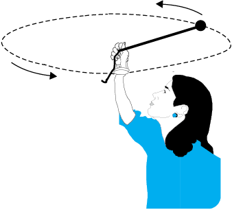
Fig. 4.4 Force is necessary for changing the direction of momentum, even if its magnitude is constant. We can feel this while rotating a stone in a horizontal circle with uniform speed by means of a string.
These qualitative observations lead to the second law of motion expressed by Newton as follows :
The rate of change of momentum of a body is directly proportional to the applied force and takes place in the direction in which the force acts.
Thus, if under the action of a force F for time interval ∆t, the velocity of a body of mass m changes from v to v + ∆v i.e. its initial momentum p = m v changes by  . According to the Second Law,
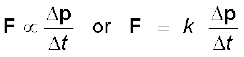
where k is a constant of proportionality. Taking the limit ∆t → 0, the term  becomes the derivative or differential co-efficient of p with respect to t, denoted by
  . Thus
 (4.2)
(4.2)
For a body of fixed mass m,
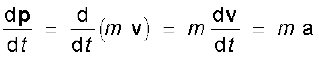 (4.3)
(4.3)
i.e the Second Law can also be written as
F = k m a (4.4)
which shows that force is proportional to the product of mass m and acceleration a.
The unit of force has not been defined so far. In fact, we use Eq. (4.4) to define the unit of force. We, therefore, have the liberty to choose any constant value for k. For simplicity, we choose k = 1. The second law then is
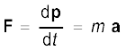 (4.5)
(4.5)
In SI unit force is one that causes an acceleration of 1 m s-2 to a mass of 1 kg. This unit is known as newton : 1 N = 1 kg m s-2.
Let us note at this stage some important points about the second law :
1. In the second law, F = 0 implies a = 0. The second law is obviously consistent with the first law.
2. The second law of motion is a vector law. It is equivalent to three equations, one for each component of the vectors :
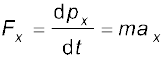
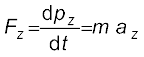 (4.6)
(4.6)
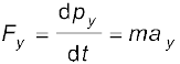
This means that if a force is not parallel to the velocity of the body, but makes some angle with it, it changes only the component of velocity along the direction of force. The component of velocity normal to the force remains unchanged. For example, in the motion of a projectile under the vertical gravitational force, the horizontal component of velocity remains unchanged (Fig. 4.5).
3. The second law of motion given by Eq. (4.5) is applicable to a single point particle. The force F in the law stands for the net external force on the particle and a stands for acceleration of the particle. It turns out, however, that the law in the same form applies to a rigid body or, even more generally, to a system of particles. In that case, F refers to the total external force on the system and a refers to the acceleration of the system as a whole. More precisely, a is the acceleration of the centre of mass of the system about which we shall study in detail in chapter 6. Any internal forces in the system are not to be included in F.
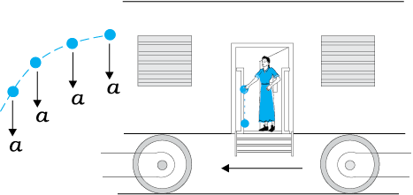
Fig. 4.5 Acceleration at an instant is determined by the force at that instant. The moment after a stone is dropped out of an accelerated train, it has no horizontal acceleration or force, if air resistance is neglected. The stone carries no memory of its acceleration with the train a moment ago.
4. The second law of motion is a local relation which means that force F at a point in space (location of the particle) at a certain instant of time is related to a at that point at that instant. Acceleration here and now is determined by the force here and now, not by any history of the motion of the particle (See Fig. 4.5).
Example 4.2 A bullet of mass 0.04 kg moving with a speed of 90 m s–1 enters a heavy wooden block and is stopped after a distance of 60 cm. What is the average resistive force exerted by the block on the bullet?
Answer The retardation ‘a’ of the bullet (assumed constant) is given by
 =
= 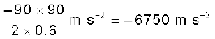
The retarding force, by the second law of motion, is
= 0.04 kg × 6750 m s-2 = 270 N
The actual resistive force, and therefore, retardation of the bullet may not be uniform. The answer therefore, only indicates the average resistive force.
Example 4.3 The motion of a particle of mass m is described by y =  Find the force acting on the particle.
Answer We know
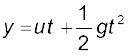
Now,
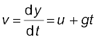
acceleration, 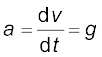
Then the force is given by Eq. (5.5)
F = ma = mg
Thus the given equation describes the motion of a particle under acceleration due to gravity and y is the position coordinate in the direction of g.
Impulse
We sometimes encounter examples where a large force acts for a very short duration producing a finite change in momentum of the body. For example, when a ball hits a wall and bounces back, the force on the ball by the wall acts for a very short time when the two are in contact, yet the force is large enough to reverse the momentum of the ball. Often, in these situations, the force and the time duration are difficult to ascertain separately. However, the product of force and time, which is the change in momentum of the body remains a measurable quantity. This product is called impulse:
Impulse = Force × time duration
= Change in momentum (4.7)
A large force acting for a short time to produce a finite change in momentum is called an impulsive force. In the history of science, impulsive forces were put in a conceptually different category from ordinary forces. Newtonian mechanics has no such distinction. Impulsive force is like any other force – except that it is large and acts for a short time.
Example 4.4 A batsman hits back a ball straight in the direction of the bowler without changing its initial speed of 12 m s–1.
If the mass of the ball is 0.15 kg, determine the impulse imparted to the ball. (Assume linear motion of the ball)
Answer Change in momentum
= 0.15 × 12–(–0.15×12)
= 3.6 N s,
Impulse = 3.6 N s,
in the direction from the batsman to the bowler.
This is an example where the force on the ball by the batsman and the time of contact of the ball and the bat are difficult to know, but the impulse is readily calculated.
4.6 Newton’s Third Law of motion
The second law relates the external force on a body to its acceleration. What is the origin of the external force on the body ? What agency provides the external force ? The simple answer in Newtonian mechanics is that the external force on a body always arises due to some other body. Consider a pair of bodies A and B. B gives rise to an external force on A. A natural question is: Does A in turn give rise to an external force on B ? In some examples, the answer seems clear. If you press a coiled spring, the spring is compressed by the force of your hand. The compressed spring in turn exerts a force on your hand and you can feel it. But what if the bodies are not in contact ? The earth pulls a stone downwards due to gravity. Does the stone exert a force on the earth ? The answer is not obvious since we hardly see the effect of the stone on the earth. The answer according to Newton is: Yes, the stone does exert an equal and opposite force on the earth. We do not notice it since the earth is very massive and the effect of a small force on its motion is negligible.
Thus, according to Newtonian mechanics, force never occurs singly in nature. Force is the mutual interaction between two bodies. Forces always occur in pairs. Further, the mutual forces between two bodies are always equal and opposite. This idea was expressed by Newton in the form of the third law of motion.
To every action, there is always an equal and opposite reaction.
Newton’s wording of the third law is so crisp and beautiful that it has become a part of common language. For the same reason perhaps, misconceptions about the third law abound. Let us note some important points about the third law, particularly in regard to the usage of the terms : action and reaction.
1. The terms action and reaction in the third law mean nothing else but ‘force’. Using different terms for the same physical concept can sometimes be confusing. A simple and clear way of stating the third law is as follows:
Forces always occur in pairs. Force on a body A by B is equal and opposite to the force on the body B by A.
2. The terms action and reaction in the third law may give a wrong impression that action comes before reaction i.e action is the cause and reaction the effect. There is no cause-effect relation implied in the third law. The force on A by B and the force on B by A act at the same instant. By the same reasoning, any one of them may be called action and the other reaction.
3. Action and reaction forces act on different bodies, not on the same body. Consider a pair of bodies A and B. According to the third law,
FAB = – FBA (4.8)
(force on A by B) =