Table of Contents
Chapter Seven
Gravitation

7.1 Introduction
7.2 Kepler’s laws
7.3 Universal law of gravitation
7.4 The gravitational constant
7.5 Acceleration due to gravity of the earth
7.6 Acceleration due to gravity below and above the surface of earth
7.7 Gravitational potential energy
7.8 Escape speed
7.9 Earth satellites
7.10 Energy of an orbiting satellite
Summary
Points to ponder
Exercises
Additional exercises
7.1 Introduction
Early in our lives, we become aware of the tendency of all material objects to be attracted towards the earth. Anything thrown up falls down towards the earth, going uphill is lot more tiring than going downhill, raindrops from the clouds above fall towards the earth and there are many other such phenomena. Historically it was the Italian Physicist Galileo (1564-1642) who recognised the fact that all bodies, irrespective of their masses, are accelerated towards the earth with a constant acceleration. It is said that he made a public demonstration of this fact. To find the truth, he certainly did experiments with bodies rolling down inclined planes and arrived at a value of the acceleration due to gravity which is close to the more accurate value obtained later.
A seemingly unrelated phenomenon, observation of stars, planets and their motion has been the subject of attention in many countries since the earliest of times. Observations since early times recognised stars which appeared in the sky with positions unchanged year after year. The more interesting objects are the planets which seem to have regular motions against the background of stars. The earliest recorded model for planetary motions proposed by Ptolemy about 2000 years ago was a ‘geocentric’ model in which all celestial objects, stars, the sun and the planets, all revolved around the earth. The only motion that was thought to be possible for celestial objects was motion in a circle. Complicated schemes of motion were put forward by Ptolemy in order to describe the observed motion of the planets. The planets were described as moving in circles with the centre of the circles themselves moving in larger circles. Similar theories were also advanced by Indian astronomers some 400 years later. However a more elegant model in which the Sun was the centre around which the planets revolved – the ‘heliocentric’ model – was already mentioned by Aryabhatta (5th century A.D.) in his treatise. A thousand years later, a Polish monk named Nicolas Copernicus (1473-1543) proposed a definitive model in which the planets moved in circles around a fixed central sun. His theory was discredited by the church, but notable amongst its supporters was Galileo who had to face prosecution from the state for his beliefs.
It was around the same time as Galileo, a nobleman called Tycho Brahe (1546-1601) hailing from Denmark, spent his entire lifetime recording observations of the planets with the naked eye. His compiled data were analysed later by his assistant Johannes Kepler (1571-1640). He could extract from the data three elegant laws that now go by the name of Kepler’s laws. These laws were known to Newton and enabled him to make a great scientific leap in proposing his universal law of gravitation.
7.2 Kepler’s laws
The three laws of Kepler can be stated as follows:
1. Law of orbits : All planets move in elliptical orbits with the Sun situated at one of the foci
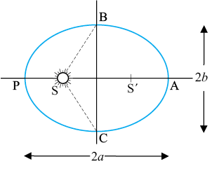
Fig. 7.1(a) An ellipse traced out by a planet around the sun. The closest point is P and the farthest point is A, P is called the perihelion and A the aphelion. The semimajor axis is half the distance AP.
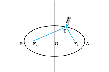
Fig. 7.1(b) Drawing an ellipse. A string has its ends fixed at F1 and F2. The tip of a pencil holds the string taut and is moved around.
of the ellipse (Fig. 7.1a). This law was a deviation from the Copernican model which allowed only circular orbits. The ellipse, of which the circle is a special case, is a closed curve which can be drawn very simply as follows.
*Refer to information given in the Box on Page 182
Select two points F1 and F2. Take a length of a string and fix its ends at F1 and F2 by pins. With the tip of a pencil stretch the string taut and then draw a curve by moving the pencil keeping the string taut throughout.(Fig. 7.1(b)) The closed curve you get is called an ellipse. Clearly for any point T on the ellipse, the sum of the distances from F1 and F2 is a constant. F1, F2 are called the focii. Join the points F1 and F2 and extend the line to intersect the ellipse at points P and A as shown in Fig. 7.1(b). The midpoint of the line PA is the centre of the ellipse O and the length PO = AO is called the semi-major axis of the ellipse. For a circle, the two focii merge into one and the semi-major axis becomes the radius of the circle.
2. Law of areas : The line that joins any planet to the sun sweeps equal areas in equal intervals of time (Fig. 7.2). This law comes from the observations that planets appear to move slower when they are farther from the sun than when they are nearer.
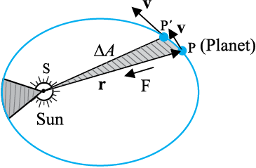
Fig. 7.2 The planet P moves around the sun in an elliptical orbit. The shaded area is the area ∆A swept out in a small interval of time ∆t.
3. Law of periods : The square of the time period of revolution of a planet is proportional to the cube of the semi-major axis of the ellipse traced out by the planet.
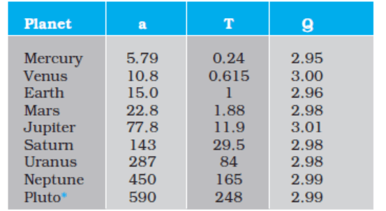
Table 7.1 gives the approximate time periods of revolution of eight* planets around the sun along with values of their semi-major axes.
Table 7.1 Data from measurement of planetary motions given below confirm Kepler’s Law of Periods
(a ≡ Semi-major axis in units of 1010 m.
T ≡ Time period of revolution of the planet in years(y).
Q ≡ The quotient ( T2/a3 ) in units of 10 -34 y2 m-3.)
The law of areas can be understood as a consequence of conservation of angular momentum whch is valid for any central force . A central force is such that the force on the planet is along the vector joining the Sun and the planet. Let the Sun be at the origin and let the position and momentum of the planet be denoted by r and p respectively. Then the area swept out by the planet of mass m in time interval ∆t is (Fig. 7.2) ∆A given by
 = ½ (r × v∆t) (7.1)
Hence
 /∆t =½ (r × p)/m, (since v = p/m)
= L / (2 m) (7.2)
where v is the velocity, L is the angular momentum equal to ( r × p). For a central force, which is directed along r, L is a constant as the planet goes around. Hence,  /∆t is a constant according to the last equation. This is the law of areas. Gravitation is a central force and hence the law of areas follows.
Johannes Kepler (1571–1630)
was a scientist of German origin. He formulated the three laws of planetary motion based on the painstaking observations of Tycho Brahe and coworkers. Kepler himself was an assistant to Brahe and it took him sixteen long years to arrive at the three planetary laws. He is also known as the founder of geometrical optics, being the first to describe what happens to light after it enters a telescope.
Example 7.1 Let the speed of the planet at the perihelion P in Fig. 7.1(a) be vP and the Sun-planet distance SP be rP. Relate {rP, vP} to the corresponding quantities at the aphelion {rA, vA}. Will the planet take equal times to traverse BAC and CPB ?
Answer The magnitude of the angular momentum at P is Lp = mp rp vp, since inspection tells us that rp and vp are mutually perpendicular. Similarly, LA = mp rA vA. From angular momentum conservation
mp rp vp = mp rA vA
or 
Since rA > rp, vp > vA .
The area SBAC bounded by the ellipse and the radius vectors SB and SC is larger than SBPC in Fig. 8.1. From Kepler’s second law, equal areas are swept in equal times. Hence the planet will take a longer time to traverse BAC than CPB.
7.3 Universal law of gravitation
Legend has it that observing an apple falling from a tree, Newton was inspired to arrive at an universal law of gravitation that led to an explanation of terrestrial gravitation as well as of Kepler’s laws. Newton’s reasoning was that the moon revolving in an orbit of radius Rm was subject to a centripetal acceleration due to earth’s gravity of magnitude
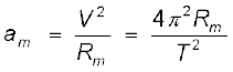 (7.3)
(7.3)
where V is the speed of the moon related to the time period T by the relation 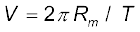 . The time period T is about 27.3 days and Rm was already known then to be about 3.84 × 10⁸m. If we substitute these numbers in Eq. (7.3), we get a value of am much smaller than the value of acceleration due to gravity g on the surface of the earth, arising also due to earth’s gravitational attraction.
 ; g α
; g α  and we get

 3600 (7.4)
in agreement with a value of g  9.8 m s-2 and the value of am from Eq. (7.3). These observations led Newton to propose the following Universal Law of Gravitation :
Every body in the universe attracts every other body with a force which is directly proportional to the product of their masses and inversely proportional to the square of the distance between them.
The quotation is essentially from Newton’s famous treatise called ‘Mathematical Principles of Natural Philosophy’ (Principia for short).
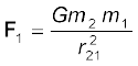
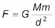
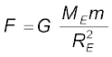
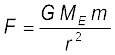
Stated Mathematically, Newton’s gravitation law reads : The force F on a point mass m2 due to another point mass m1 has the magnitude
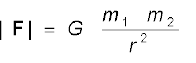 (7.5)
(7.5)
Equation (7.5) can be expressed in vector form as
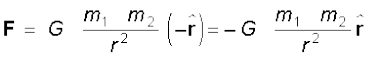
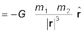
where G is the universal gravitational constant,  is the unit vector from m1 to m2 and r = r2 – r1 as shown in Fig. 7.3.
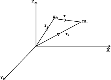
Fig. 7.3 Gravitational force on m1 due to m2 is along r where the vector r is (r2– r1).
The gravitational force is attractive, i.e., the force F is along – r. The force on point mass m1 due to m2 is of course – F by Newton’s third law. Thus, the gravitational force F12 on the body 1 due to 2 and F21 on the body 2 due to 1 are related as F12 = – F21.
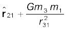
Before we can apply Eq. (7.5) to objects under consideration, we have to be careful since the law refers to point masses whereas we deal with extended objects which have finite size. If we have a collection of point masses, the force on any one of them is the vector sum of the gravitational forces exerted by the other point masses as shown in Fig 7.4.
Fig. 7.4 Gravitational force on point mass m1 is the vector sum of the gravitational forces exerted by m2, m3 and m4.
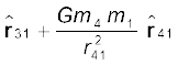
The total force on m1 is
Example 7.2 Three equal masses of m kg each are fixed at the vertices of an equilateral triangle ABC.
(a) What is the force acting on a mass 2m placed at the centroid G of the triangle?
(b) What is the force if the mass at the vertex A is doubled ?
Take AG = BG = CG = 1 m (see Fig. 7.5)
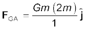
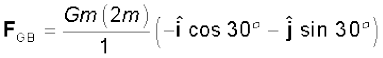
Answer (a) The angle between GC and the positive x-axis is 30° and so is the angle between GB and the negative x-axis. The individual forces in vector notation are
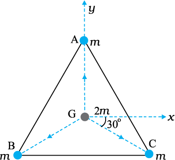
Fig. 7.5 Three equal masses are placed at the three vertices of the ∆ ABC. A mass 2m is placed at the centroid G.

From the principle of superposition and the law of vector addition, the resultant gravitational force FR on (2m) is
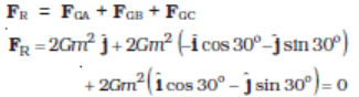
Alternatively, one expects on the basis of symmetry that the resultant force ought to be zero.
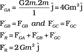
(b) Now if the mass at vertex A is doubled then
For the gravitational force between an extended object (like the earth) and a point mass, Eq. (8.5) is not directly applicable. Each point mass in the extended object will exert a force on the given point mass and these force will not all be in the same direction. We have to add up these forces vectorially for all the point masses in the extended object to get the total force. This is easily done using calculus. For two special cases, a simple law results when you do that :
(1) The force of attraction between a hollow spherical shell of uniform density and a point mass situated outside is just as if the entire mass of the shell is concentrated at the centre of the shell.
Qualitatively this can be understood as follows: Gravitational forces caused by the various regions of the shell have components along the line joining the point mass to the centre as well as along a direction prependicular to this line. The components prependicular to this line cancel out when summing over all regions of the shell leaving only a resultant force along the line joining the point to the centre. The magnitude of this force works out to be as stated above.
Newton’s Principia
Kepler had formulated his third law by 1619. The announcement of the underlying universal law of gravitation came about seventy years later with the publication in 1687 of Newton’s masterpiece Philosophiae Naturalis Principia Mathematica, often simply called the Principia.
Around 1685, Edmund Halley (after whom the famous Halley’s comet is named), came to visit Newton at Cambridge and asked him about the nature of the trajectory of a body moving under the influence of an inverse square law. Without hesitation Newton replied that it had to be an ellipse, and further that he had worked it out long ago around 1665 when he was forced to retire to his farm house from Cambridge on account of a plague outbreak. Unfortunately, Newton had lost his papers. Halley prevailed upon Newton to produce his work in book form and agreed to bear the cost of publication. Newton accomplished this feat in eighteen months of superhuman effort. The Principia is a singular scientific masterpiece and in the words of Lagrange it is “the greatest production of the human mind.” The Indian born astrophysicist and Nobel laureate S. Chandrasekhar spent ten years writing a treatise on the Principia. His book, Newton’s Principia for the Common Reader brings into sharp focus the beauty, clarity and breath taking economy of Newton’s methods.
(2) The force of attraction due to a hollow spherical shell of uniform density, on a point mass situated inside it is zero.
Qualitatively, we can again understand this result. Various regions of the spherical shell attract the point mass inside it in various directions. These forces cancel each other completely.
7.4 The Gravitational Constant
The value of the gravitational constant G entering the Universal law of gravitation can be determined experimentally and this was first done by English scientist Henry Cavendish in 1798. The apparatus used by him is schematically shown in figure.7.6
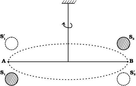
Fig. 7.6 Schematic drawing of Cavendish’s experiment. S1 and S2 are large spheres which are kept on either side (shown shades) of the masses at A and B. When the big spheres are taken to the other side of the masses (shown by dotted circles), the bar AB rotates a little since the torque reverses direction. The angle of rotation can be measured experimentally.
The bar AB has two small lead spheres attached at its ends. The bar is suspended from a rigid support by a fine wire. Two large lead spheres are brought close to the small ones but on opposite sides as shown. The big spheres attract the nearby small ones by equal and opposite force as shown. There is no net force on the bar but only a torque which is clearly equal to F times the length of the bar,where F is the force of attraction between a big sphere and its neighbouring small sphere. Due to this torque, the suspended wire gets twisted till such time as the restoring torque of the wire equals the gravitational torque . If θ is the angle of twist of the suspended wire, the restoring torque is proportional to θ, equal to τθ. Where τ is the restoring couple per unit angle of twist. τ can be measured independently e.g. by applying a known torque and measuring the angle of twist. The gravitational force between the spherical balls is the same as if their masses are concentrated at their centres. Thus if d is the separation between the centres of the big and its neighbouring small ball, M and m their masses, the gravitational force between the big sphere and its neighouring small ball is.
 (7.6)
(7.6)
If L is the length of the bar AB , then the torque arising out of F is F multiplied by L. At equilibrium, this is equal to the restoring torque and hence
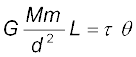 (7.7)
(7.7)
Observation of θ thus enables one to calculate G from this equation.
Since Cavendish’s experiment, the measurement of G has been refined and the currently accepted value is
G = 6.67×10⁻¹¹ N m2/kg2 (7.8)
7.5 Acceleration due to gravity of the earth
The earth can be imagined to be a sphere made of a large number of concentric spherical shells with the smallest one at the centre and the largest one at its surface. A point outside the earth is obviously outside all the shells. Thus, all the shells exert a gravitational force at the point outside just as if their masses are concentrated at their common centre according to the result stated in section 7.3. The total mass of all the shells combined is just the mass of the earth. Hence, at a point outside the earth, the gravitational force is just as if its entire mass of the earth is concentrated at its centre.
For a point inside the earth, the situation is different. This is illustrated in Fig. 7.7.
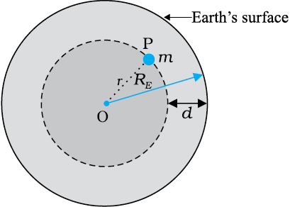
Fig. 7.7 The mass m is in a mine located at a depth d below the surface of the Earth of mass ME and radius RE. We treat the Earth to be spherically symmetric.
Again consider the earth to be made up of concentric shells as before and a point mass m situated at a distance r from the centre. The point P lies outside the sphere of radius r. For the shells of radius greater than r, the point P lies inside. Hence according to result stated in the last section, they exert no gravitational force on mass m kept at P. The shells with radius  r make up a sphere of radius r for which the point P lies on the surface. This smaller sphere therefore exerts a force on a mass m at P as if its mass Mr is concentrated at the centre. Thus the force on the mass m at P has a magnitude
 (7.9)
(7.9)
We assume that the entire earth is of uniform density and hence its mass is 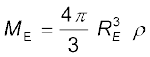 where ME is the mass of the earth RE is its radius and ρ is the density. On the other hand the mass of the sphere Mr of radius r is
  and hence
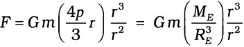
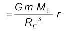 (7.10)
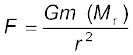
If the mass m is situated on the surface of earth, then r = RE and the gravitational force on it is, from Eq. (7.10)
 (7.11)
The acceleration experienced by the mass m, which is usually denoted by the symbol g is related to F by Newton’s 2nd law by relation
F = mg. Thus
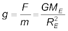 (7.12)
Acceleration g is readily measurable. RE is a known quantity. The measurement of G by Cavendish’s experiment (or otherwise), combined with knowledge of g and RE enables one to estimate ME from Eq. (7.12). This is the reason why there is a popular statement regarding Cavendish : “Cavendish weighed the earth”.
7.6 Acceleration due to gravity below and above the surface of earth
Consider a point mass m at a height h above the surface of the earth as shown in Fig. 8.8(a). The radius of the earth is denoted by RE . Since this point is outside the earth,
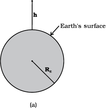
Fig. 7.8 (a) g at a height h above the surface of the earth.
its distance from the centre of the earth is (RE + h ). If F (h) denoted the magnitude of the force on the point mass m , we get from Eq. (7.5) :
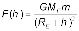 (7.13)
The acceleration experienced by the point mass is 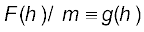 and we get
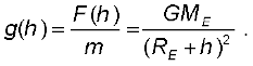 (7.14)
This is clearly less than the value of g on the surface of earth : 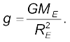 For
For  we can expand the RHS of Eq. (7.14) :
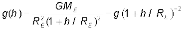
For  , using binomial expression,
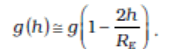 . (7.15)
Equation (7.15) thus tells us that for small heights h above the value of g decreases by a factor 
Now, consider a point mass m at a depth d below the surface of the earth (Fig. 7.8(b)), so that its distance from the centre of the earth is  as shown in the figure. The earth can be thought of as being composed of a smaller sphere of radius (RE – d ) and a spherical shell of thickness d. The force on m due to the outer shell of thickness d is zero because the result quoted in the previous section. As far as the smaller sphere of radius ( RE – d ) is concerned, the point mass is outside it and hence according to the result quoted earlier, the force due to this smaller sphere is just as if the entire mass of the smaller sphere is concentrated at the centre. If Ms is the mass of the smaller sphere, then,
Ms/ME = ( RE – d)3 / RE3 ( 7.16)
Since mass of a sphere is proportional to be cube of its radius.
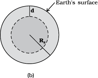
Fig. 7.8 (b) g at a depth d. In this case only the smaller sphere of radius (RE–d) contributes to g.
Thus the force on the point mass is
F (d) = G Ms m / (RE – d ) 2 (7.17)
Substituting for Ms from above , we get
F (d) = G ME m ( RE – d ) / RE 3 (7.18)
and hence the acceleration due to gravity at a depth d,
g(d) =  is
is
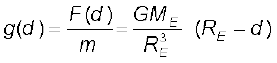
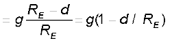 (7.19)
Thus, as we go down below earth’s surface, the acceleration due gravity decreases by a factor  The remarkable thing about acceleration due to earth’s gravity is that it is maximum on its surface decreasing whether you go up or down.
7.7 Gravitational potential energy
We had discussed earlier the notion of potential energy as being the energy stored in the body at its given position. If the position of the particle changes on account of forces acting on it, then the change in its potential energy is just the amount of work done on the body by the force. As we had discussed earlier, forces for which the work done is independent of the path are the conservative forces.
The force of gravity is a conservative force and we can calculate the potential energy of a body arising out of this force, called the gravitational potential energy. Consider points close to the surface of earth, at distances from the surface much smaller than the radius of the earth. In such cases, the force of gravity is practically a constant equal to mg, directed towards the centre of the earth. If we consider a point at a height h1 from the surface of the earth and another point vertically above it at a height h2 from the surface, the work done in lifting the particle of mass m from the first to the second position is denoted by W12
W12 = Force × displacement
= mg (h2 – h1) (7.20)
If we associate a potential energy W(h) at a point at a height h above the surface such that
W(h) = mgh + Wo (7.21)
(where Wo = constant) ;
then it is clear that
W12 = W(h2) – W(h1) (7.22)
The work done in moving the particle is just the difference of potential energy between its final and initial positions.Observe that the constant Wo cancels out in Eq. (7.22). Setting h = 0 in the last equation, we get W ( h = 0 ) = Wo. . h = 0 means points on the surface of the earth. Thus, Wo is the potential energy on the surface of the earth.
If we consider points at arbitrary distance from the surface of the earth, the result just derived is not valid since the assumption that the gravitational force mg is a constant is no longer valid. However, from our discussion we know that a point outside the earth, the force of gravitation on a particle directed towards the centre of the earth is
 (7.23)
where ME = mass of earth, m = mass of the particle and r its distance from the centre of the earth. If we now calculate the work done in lifting a particle from r = r1 to r = r2 (r2 > r1) along a vertical path, we get instead of Eq. (7.20)
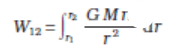
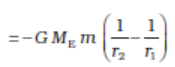 (7.24)
In place of Eq. (7.21), we can thus associate a potential energy W(r) at a distance r, such that
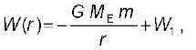 (7.25)
valid for r > R ,
so that once again W12 = W(r2) – W(r1). Setting r = infinity in the last equation, we get W ( r = infinity ) = W1 . Thus, W1 is the potential energy at infinity. One should note that only the difference of potential energy between two points has a definite meaning from Eqs. (8.22) and (8.24). One conventionally sets W1 equal to zero, so that the potential energy at a point is just the amount of work done in displacing the particle from infinity to that point.
We have calculated the potential energy at a point of a particle due to gravitational forces on it due to the earth and it is proportional to the mass of the particle. The gravitational potential due to the gravitational force of the earth is defined as the potential energy of a particle of unit mass at that point. From the earlier discussion, we learn that the gravitational potential energy associated with two particles of masses m1 and m2 separated by distance by a distance r is given by
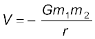 (if we choose V = 0 as r
  )
)
It should be noted that an isolated system of particles will have the total potential energy that equals the sum of energies (given by the above equation) for all possible pairs of its constituent particles. This is an example of the application of the superposition principle.
Example 7.3 Find the potential energy of a system of four particles placed at the vertices of a square of side l. Also obtain the potential at the centre of the square.
Answer Consider four masses each of mass m at the corners of a square of side l; See Fig. 8.9. We have four mass pairs at distance l and two diagonal pairs at distance 
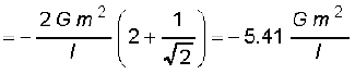
Hence,
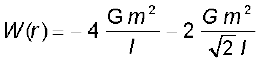
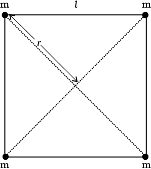
Fig. 7.9
The gravitational potential at the centre of the square 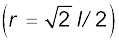 is
is
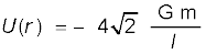 .
.
7.8 Escape Speed
If a stone is thrown by hand, we see it falls back to the earth. Of course using machines we can shoot an object with much greater speeds and with greater and greater initial