Table of Contents
CHAPTER THIRTEEN

OSCILLATIONS
13.1 Introduction
13.2 Periodic and oscillatory motions
13.3 Simple harmonic motion
13.4 Simple harmonic motion and uniform circular motion
13.5 Velocity and acceleration in simple harmonic motion
13.6 Force law for simple harmonic motion
13.7 Energy in simple harmonic motion
13.8 The simple pendulum
Summary
Points to ponder
Exercises
13.1 INTRODUCTION
In our daily life we come across various kinds of motions. You have already learnt about some of them, e.g., rectilinear motion and motion of a projectile. Both these motions are non-repetitive. We have also learnt about uniform circular motion and orbital motion of planets in the solar system. In these cases, the motion is repeated after a certain interval of time, that is, it is periodic. In your childhood, you must have enjoyed rocking in a cradle or swinging on a swing. Both these motions are repetitive in nature but different from the periodic motion of a planet. Here, the object moves to and fro about a mean position. The pendulum of a wall clock executes a similar motion. Examples of such periodic to and fro motion abound: a boat tossing up and down in a river, the piston in a steam engine going back and forth, etc. Such a motion is termed as oscillatory motion. In this chapter we study this motion.
The study of oscillatory motion is basic to physics; its concepts are required for the understanding of many physical phenomena. In musical instruments, like the sitar, the guitar or the violin, we come across vibrating strings that produce pleasing sounds. The membranes in drums and diaphragms in telephone and speaker systems vibrate to and fro about their mean positions. The vibrations of air molecules make the propagation of sound possible. In a solid, the atoms vibrate about their equilibrium positions, the average energy of vibrations being proportional to temperature. AC power supply give voltage that oscillates alternately going positive and negative about the mean value (zero).
The description of a periodic motion, in general, and oscillatory motion, in particular, requires some fundamental concepts, like period, frequency, displacement, amplitude and phase. These concepts are developed in the next section.
13.2 Periodic and Oscillatory motions
Fig. 13.1 shows some periodic motions. Suppose an insect climbs up a ramp and falls down, it comes back to the initial point and repeats the process identically. If you draw a graph of its height above the ground versus time, it would look something like Fig. 13.1 (a). If a child climbs up a step, comes down, and repeats the process identically, its height above the ground would look like that in Fig. 13.1 (b). When you play the game of bouncing a ball off the ground, between your palm and the ground, its height versus time graph would look like the one in Fig. 13.1 (c). Note that both the curved parts in Fig. 13.1 (c) are sections of a parabola given by the Newton’s equation of motion (see section 2.6), for downward motion, and
 for upward motion,
with different values of u in each case. These are examples of periodic motion. Thus, a motion that repeats itself at regular intervals of time is called periodic motion.
 (a)
(a)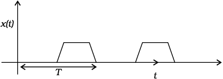 (b)
(b)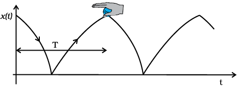 (c)
(c)Fig. 13.1 Examples of periodic motion. The period T is shown in each case.
Very often, the body undergoing periodic motion has an equilibrium position somewhere inside its path. When the body is at this position no net external force acts on it. Therefore, if it is left there at rest, it remains there forever. If the body is given a small displacement from the position, a force comes into play which tries to bring the body back to the equilibrium point, giving rise to oscillations or vibrations. For example, a ball placed in a bowl will be in equilibrium at the bottom. If displaced a little from the point, it will perform oscillations in the bowl. Every oscillatory motion is periodic, but every periodic motion need not be oscillatory. Circular motion is a periodic motion, but it is not oscillatory.
There is no significant difference between oscillations and vibrations. It seems that when the frequency is small, we call it oscillation (like, the oscillation of a branch of a tree), while when the frequency is high, we call it vibration (like, the vibration of a string of a musical instrument). Simple harmonic motion is the simplest form of oscillatory motion. This motion arises when the force on the oscillating body is directly proportional to its displacement from the mean position, which is also the equilibrium position. Further, at any point in its oscillation, this force is directed towards the mean position.
In practice, oscillating bodies eventually come to rest at their equilibrium positions because of the damping due to friction and other dissipative causes. However, they can be forced to remain oscillating by means of some external periodic agency. We discuss the phenomena of damped and forced oscillations later in the chapter.
Any material medium can be pictured as a collection of a large number of coupled oscillators. The collective oscillations of the constituents of a medium manifest themselves as waves. Examples of waves include water waves, seismic waves, electromagnetic waves. We shall study the wave phenomenon in the next chapter.
13.2.1 Period and frequency
We have seen that any motion that repeats itself at regular intervals of time is called periodic motion. The smallest interval of time after which the motion is repeated is called its period. Let us denote the period by the symbol T. Its SI unit is second. For periodic motions, which are either too fast or too slow on the scale of seconds, other convenient units of time are used. The period of vibrations of a quartz crystal is expressed in units of microseconds (10–6 s) abbreviated as µs. On the other hand, the orbital period of the planet Mercury is 88 earth days. The Halley’s comet appears after every 76 years.
The reciprocal of T gives the number of repetitions that occur per unit time. This quantity is called the frequency of the periodic motion. It is represented by the symbol ν. The relation between ν and T is
ν = 1/T (13.1)
The unit of ν is thus s–1. After the discoverer of radio waves, Heinrich Rudolph Hertz (1857–1894), a special name has been given to the unit of frequency. It is called hertz (abbreviated as Hz). Thus,
1 hertz = 1 Hz =1 oscillation per second =1s–1 (13.2)
Note, that the frequency, ν, is not necessarily an integer.
Example 13.1 On an average, a human heart is found to beat 75 times in a minute. Calculate its frequency and period.
Answer The beat frequency of heart = 75/(1 min)
= 75/(60 s)
= 1.25 s–1
= 1.25 Hz
The time period T = 1/(1.25 s–1)
= 0.8 s
13.2.2 Displacement
In section 3.2, we defined displacement of a particle as the change in its position vector. In this chapter, we use the term displacement in a more general sense. It refers to change with time of any physical property under consideration. For example, in case of rectilinear motion of a steel ball on a surface, the distance from the starting point as a function of time is its position displacement. The choice of origin is a matter of convenience. Consider a block attached to a spring, the other end of the spring is fixed to a rigid wall [see Fig.13.2(a)]. Generally, it is convenient to measure displacement of the body from its equilibrium position. For an oscillating simple pendulum, the angle from the vertical as a function of time may be regarded as a displacement variable [see Fig.13.2(b)]. The term displacement is not always to be referred in the context of position only. There can be many other kinds of displacement variables. The voltage across a capacitor, changing with time in an AC circuit, is also a displacement variable. In the same way, pressure variations in time in the propagation of sound wave, the changing electric and magnetic fields in a light wave are examples of displacement in different contexts. The displacement variable may take both positive and negative values. In experiments on oscillations, the displacement is measured for different times.
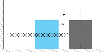
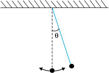
Fig.13.2(b) An oscillating simple pendulum; its motion can be described in terms of angular displacement θ from the vertical.
The displacement can be represented by a mathematical function of time. In case of periodic motion, this function is periodic in time. One of the simplest periodic functions is given by
f (t) = A cos ωt (13.3a)
If the argument of this function, ωt, is increased by an integral multiple of 2π radians, the value of the function remains the same. The function f (t) is then periodic and its period, T, is given by
 (13.3b)
Thus, the function f (t) is periodic with period T,
f (t) = f (t+T )
The same result is obviously correct if we consider a sine function, f (t ) = A sin ωt. Further, a linear combination of sine and cosine functions like,
f (t) = A sin ωt + B cos ωt (13.3c)
is also a periodic function with the same period T. Taking,
A = D cos φ and B = D sin φ
Eq. (13.3c) can be written as,
f (t) = D sin (ωt + φ ) , (13.3d)
Here D and φ are constant given by
 (B/A)
(B/A)
The great importance of periodic sine and cosine functions is due to a remarkable result proved by the French mathematician, Jean Baptiste Joseph Fourier (1768–1830): Any periodic function can be expressed as a superposition of sine and cosine functions of different time periods with suitable coefficients.
Example 13.2 Which of the following functions of time represent (a) periodic and (b) non-periodic motion? Give the period for each case of periodic motion [ω is any positive constant].
(i) sin ωt + cos ωt
(ii) sin ωt + cos 2 ωt + sin 4 ωt
(iii) e–ωt
(iv) log (ωt)
Answer
(i) sin ωt + cos ωt is a periodic function, it can also be written as  sin (ωt + π/4).
Now sin (ωt + π/4)=
 sin (ωt + π/4+2π)
=  sin [ω (t + 2π/ω) + π/4]
The periodic time of the function is 2π/ω.
(ii) This is an example of a periodic motion. It can be noted that each term represents a periodic function with a different angular frequency. Since period is the least interval of time after which a function repeats its value, sin ωt has a period T0= 2π/ω ; cos 2 ωt has a period π/ω =T0/2; and sin 4 ωt has a period 2π/4ω = T0/4. The period of the first term is a multiple of the periods of the last two terms. Therefore, the smallest interval of time after which the sum of the three terms repeats is T0, and thus, the sum is a periodic function with a period 2π/ω.
(iii) The function e–ωt is not periodic, it decreases monotonically with increasing time and tends to zero as t → ∞ and thus, never repeats its value.
(iv) The function log(ωt) increases monotonically with time t. It, therefore, never repeats its value and is a non-periodic function. It may be noted that as
t → ∞, log(ωt) diverges to ∞. It, therefore, cannot represent any kind of physical displacement.
13.3 Simple harmonic motion
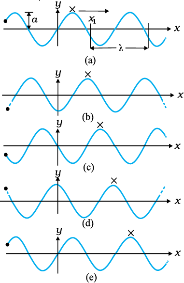
Consider a particle oscillating back and forth about the origin of an x-axis between the limits +A and –A as shown in Fig. 13.3. This oscillatory motion is said to be simple harmonic if the displacement x of the particle from the origin varies with time as :
x (t) = A cos (ω t + φ) (13.4)

Fig. 13.3 A particle vibrating back and forth about the origin of x-axis, between the limits+A and –A.
where A, ω and φ are constants.
Thus, simple harmonic motion (SHM) is not any periodic motion but one in which displacement is a sinusoidal function of time. Fig. 13.4 shows the positions of a particle executing SHM at discrete value of time, each interval of time being T/4, where T is the period of motion. Fig. 13.5 plots the graph of x versus t, which gives the values of displacement as a continuous function of time. The quantities A, ω and φ which characterize a given SHM have standard names, as summarised in Fig. 13.6. Let us understand these quantities.
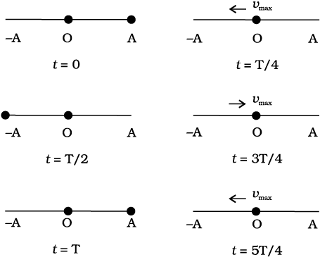
Fig. 13.4 The location of the particle in SHM at the discrete values t = 0, T/4, T/2, 3T/4, T,5T/4. The time after which motion repeats itself is T. T will remain fixed, no matter whatlocation you choose as the initial (t = 0) location. The speed is maximum for zerodisplacement (at x = 0) and zero at the extremes of motion.
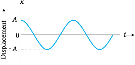
Fig. 13.5 Displacement as a continuous function of time for simple harmonic motion.
x (t) : displacement x as a function of time t
A : amplitude
ω : angular frequency
ωt + φ : phase (time-dependent)
φ : phase constant
Fig. 13.6 The meaning of standard symbols in Eq. (13.4)
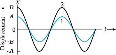
The amplitutde A of SHM is the magnitude of maximum displacement of the particle. [Note, A can be taken to be positive without any loss of generality]. As the cosine function of time varies from +1 to –1, the displacement varies between the extremes A and – A. Two simple harmonic motions may have same ω and φ but different amplitudes A and B, as shown in Fig. 13.7 (a).
While the amplitude A is fixed for a given SHM, the state of motion (position and velocity) of the particle at any time t is determined by the argument (ωt + φ) in the cosine function. This time-dependent quantity, (ωt + φ) is called the phase of the motion. The value of plase at t = 0 is φ and is called the phase constant (or phase angle). If the amplitude is known, φ can be determined from the displacement at t = 0. Two simple harmonic motions may have the same A and ω but different phase angle φ, as shown in Fig. 13.7 (b).
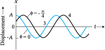
Fig. 13.7 (b) A plot obtained from Eq. (13.4). The curves 3 and 4 are for φ = 0 and -π/4respectively. The amplitude A is same for both the plots.
Finally, the quantity ω can be seen to be related to the period of motion T. Taking, for simplicity, φ = 0 in Eq. (13.4), we have
x(t) = A cos ωt (13.5)
Since the motion has a period T, x (t) is equal to x (t + T). That is,
A cos ωt = A cos ω (t + T) (13.6)
Now the cosine function is periodic with period 2π, i.e., it first repeats itself when the argument changes by 2π. Therefore,
ω(t + T ) = ωt + 2π
that is ω = 2π/ T (13.7)
ω is called the angular frequency of SHM. Its S.I. unit is radians per second. Since the frequency of oscillations is simply 1/T, ω is 2π times the frequency of oscillation. Two simple harmonic motions may have the same A and φ, but different ω, as seen in Fig. 13.8. In this plot the curve (b) has half the period and twice the frequency of the curve (a).
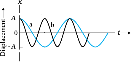
Fig. 13.8 Plots of Eq. (13.4) for φ = 0 for two different periods.
Example 13.3 Which of the following functions of time represent (a) simple harmonic motion and (b) periodic but not simple harmonic? Give the period for each case.
(1) sin ωt – cos ωt
(2) sin2 ωt
Answer
(a) sin ωt – cos ωt
= sin ωt – sin (π/2 – ωt)
= 2 cos (π/4) sin (ωt – π/4)
= √2 sin (ωt – π/4)
This function represents a simple harmonic motion having a period T = 2π/ω and a phase angle (–π/4) or (7π/4)
(b) sin2 ωt
= ½ – ½ cos 2 ωt
The function is periodic having a period T = π/ω. It also represents a harmonic motion with the point of equilibrium occurring at ½ instead of zero.
13.4 Simple harmonic motion and uniform circular motion
In this section, we show that the projection of uniform circular motion on a diameter of the circle follows simple harmonic motion. A simple experiment (Fig. 13.9) helps us visualise this connection. Tie a ball to the end of a string and make it move in a horizontal plane about a fixed point with a constant angular speed. The ball would then perform a uniform circular motion in the horizontal plane. Observe the ball sideways or from the front, fixing your attention in the plane of motion. The ball will appear to execute to and fro motion along a horizontal line with the point of rotation as the midpoint. You could alternatively observe the shadow of the ball on a wall which is perpendicular to the plane of the circle. In this process what we are observing is the motion of the ball on a diameter of the circle normal to the direction of viewing.
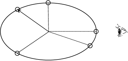
Fig. 13.9 Circular motion of a ball in a plane viewed edge-on is SHM.
Fig. 13.10 describes the same situation mathematically. Suppose a particle P is moving uniformly on a circle of radius A with angular speed ω. The sense of rotation is anticlockwise. The initial position vector of the particle, i.e., the vector  at t = 0 makes an angle of φ with the positive direction of x-axis. In time t, it will cover a further angle ωt and its position vector will make an angle of ωt + φ with the +ve x-axis. Next, consider the projection of the position vector OP on the x-axis. This will be OP′. The position of P′ on the x-axis, as the particle P moves on the circle, is given by
x(t) = A cos (ωt + φ )
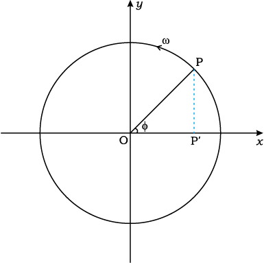
Fig.13.10
which is the defining equation of SHM. This shows that if P moves uniformly on a circle, its projection P′ on a diameter of the circle executes SHM. The particle P and the circle on which it moves are sometimes referred to as the reference particle and the reference circle, respectively.
We can take projection of the motion of P on any diameter, say the y-axis. In that case, the displacement y(t) of P′ on the y-axis is given by
y = A sin (ωt + φ)
which is also an SHM of the same amplitude as that of the projection on x-axis, but differing by a phase of π/2.
In spite of this connection between circular motion and SHM, the force acting on a particle in linear simple harmonic motion is very different from the centripetal force needed to keep a particle in uniform circular motion.
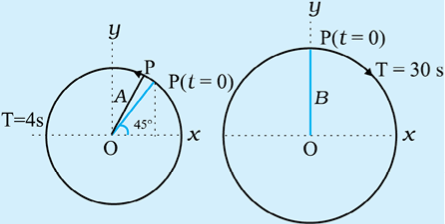
Example 13.4 The figure given below depicts two circular motions. The radius of the circle, the period of revolution, the initial position and the sense of revolution are indicated in the figures. Obtain the simple harmonic motions of the x-projection of the radius vector of the rotating particle P in each case.
Answer
(a) At t = 0, OP makes an angle of 45o = π/4 rad with the (positive direction of) x-axis. After time t, it covers an angle  in the anticlockwise sense, and makes an angle of
  with the x-axis.
The projection of OP on the x-axis at time t is given by,
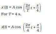
which is a SHM of amplitude A, period 4 s, and an initial phase* =  .
.
(b) In this case at t = 0, OP makes an angle of 90o =  with the x-axis. After a time t, it covers an angle of
  in the clockwise sense and makes an angle of
  with the x-axis. The projection of OP on the x-axis at time t is given by
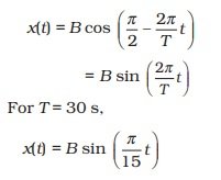
Writing this as x (t) = B cos , and comparing with Eq. (13.4). We find that this represents a SHM of amplitude B, period 30 s, and an initial phase of
  .
.
______________________________________________
*The natural unit of angle is radian, defined through the ratio of arc to radius. Angle is a dimensionless quantity. Therefore it is not always necessary to mention the unit ‘radian’ when we use π, its multiples or submultiples. The conversion between radian and degree is not similar to that between metre and centimetre or mile. If the argument of a trigonometric function is stated without units, it is understood that the unit is radian. On the other hand, if degree is to be used as the unit of angle, then it must be shown explicitly. For example, sin(150) means sine of 15 degree, but sin(15) means sine of 15 radians. Hereafter, we will often drop ‘rad’ as the unit, and it should be understood that whenever angle is mentioned as a numerical value, without units, it is to be taken as radians.
13.5 Velocity and acceleration in simple harmonic motion
The speed of a particle v in uniform circular motion is its angular speed ω times the radius of the circle A.
v = ω A (13.8)
The direction of velocity  at a time t is along the tangent to the circle at the point where the particle is located at that instant. From the geometry of Fig. 13.11, it is clear that the velocity of the projection particle P′ at time t is
v(t) = –ωA sin (ωt + φ ) (13.9)
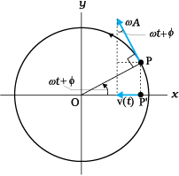
Fig. 13.11 The velocity, v (t), of the particle P′ is the projection of the velocity  of thereference particle, P.
where the negative sign shows that v (t) has a direction opposite to the positive direction of x-axis. Eq. (13.9) gives the instantaneous velocity of a particle executing SHM, where displacement is given by Eq. (13.4). We can, of course, obtain this equation without using geometrical argument, directly by differentiating (Eq. 13.4) with respect of t:
 (13.10)
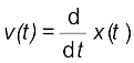
The method of reference circle can be similarly used for obtaining instantaneous acceleration of a particle undergoing SHM. We know that the centripetal acceleration of a particle P in uniform circular motion has a magnitude v2/A or ω2A, and it is directed towards the centre i.e., the direction is along PO. The instantaneous acceleration of the projection particle P′ is then (See Fig. 13.12)
a (t) = –ω2A cos (ωt + φ)
= –ω2x (t) (13.11)
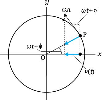
Fig. 13.12 The acceleration, a(t), of the particle P′ is the projection of the acceleration a ofthe reference particle P.
Eq. (13.11) gives the acceleration of a particle in SHM. The same equation can again be obtained directly by differentiating velocity v(t) given by Eq. (13.9) with respect to time:
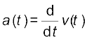 (13.12)
We note from Eq. (13.11) the important property that acceleration of a particle in SHM is proportional to displacement. For x(t) > 0, a(t) < 0 and for x(t) < 0, a(t) > 0. Thus, whatever the value of x between –A and A, the acceleration a(t) is always directed towards the centre.
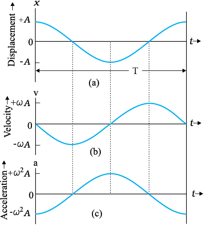
For simplicity, let us put φ = 0 and write the expression for x (t), v (t) and a(t)
x(t) = A cos ωt, v(t) = – ω Asin ωt, a(t)=–ω2 A cos ωt
The corresponding plots are shown in Fig. 13.13. All quantities vary sinusoidally with time; only their maxima differ and the different plots differ in phase. x varies between –A to A; v(t) varies from –ωA to ωA and a(t) from –ω2A to ω2A. With respect to displacement plot, velocity plot has a phase difference of π/2 and acceleration plot has a phase difference of π
Example 13.5 A body oscillates with SHM according to the equation (in SI units),
x = 5 cos [2π t + π/4].
At t = 1.5 s, calculate the (a) displacement, (b) speed and (c) acceleration of the body.
Answer The angular frequency ω of the body
= 2π s–1 and its time period T = 1 s.
At t = 1.5 s
(a) displacement = (5.0 m) cos [(2π s–1) ×
1.5 s + π/4]
= (5.0 m) cos [(3π + π/4)]
= –5.0 × 0.707 m
= –3.535 m
(b) Using Eq. (13.9), the speed of the body
= – (5.0 m)(2π s–1) sin [(2π s–1) ×1.5 s
+ π/4]
= – (5.0 m)(2π s–1) sin [(3π + π/4)]
= 10π × 0.707 m s–1
= 22 m s–1
(c) Using Eq.(13.10), the acceleration of the body
= –(2π s–1)2 × displacement
= – (2π s–1)2 × (–3.535 m)
= 140 m s–2
13.6 Force law for simple harmonic motion
Using Newton’s second law of motion, and the expression for acceleration of a particle undergoing SHM (Eq. 13.11), the force acting on a particle of mass m in SHM is
F (t) = ma
= –mω2 x (t)
i.e., F (t) = –k x (t) (13.13)
where k = mω2 (13.14a)
or  (13.14b)
Like acceleration, force is always directed towards the mean position—hence it is sometimes called the restoring force in SHM. To summarise the discussion so far, simple harmonic motion can be defined in two equivalent ways, either by Eq. (13.4) for displacement or by Eq. (13.13) that gives its force law. Going from Eq. (13.4) to Eq. (13.13) required us to differentiate two times. Likewise, by integrating the force law Eq. (13.13) two times, we can get back Eq. (13.4).
Note that the force in Eq. (13.13) is linearly proportional to x(t). A particle oscillating under such a force is, therefore, calling a linear harmonic oscillator. In the real world, the force may contain small additional terms proportional to x2, x3, etc. These then are called non-linear oscillators.
Example 13.6 Two identical springs of spring constant k are attached to a block of mass m and to fixed supports as shown in Fig. 13.13. Show that when the mass is displaced from its equilibrium position on either side, it executes a simple harmonic motion. Find the period of oscillations.
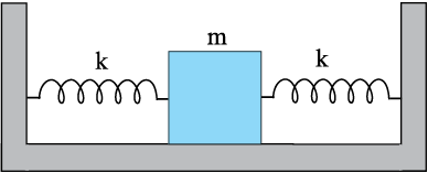
Fig. 13.14
Answer Let the mass be displaced by a small distance x to the right side of the equilibrium position, as shown in Fig. 13.15. Under this situation the spring on the left side gets elongated by a length equal to x and that on the right side gets compressed by the same length. The forces acting on the mass are then,
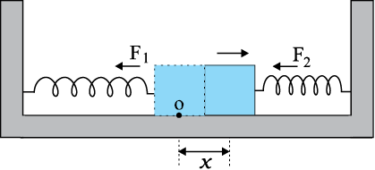
Fig. 13.15
F1 = –k x (force exerted by the spring on the left side, trying to pull the mass towards the mean position)
F2 = –k x (force exerted by the spring on the right side, trying to push the mass towards the mean position)
The net force, F, acting on the mass is then given by,
F = –2kx
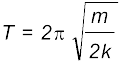
Hence the force acting on the mass is proportional to the displacement and is directed towards the mean position; therefore, the motion executed by the mass is simple harmonic. The time period of oscillations is,
13.7 Energy in simple harmonic motion
Both kinetic and potential energies of a particle in SHM vary between zero and their maximum values.
In section13.5 we have seen that the velocity of a particle executing SHM, is a periodic function of time. It is zero at the extreme positions of displacement. Therefore, the kinetic energy (K) of such a particle, which is defined as
 (13.15)
is also a periodic function of time, being zero when the displacement is maximum and maximum when the particle is at the mean position. Note, since the sign of v is immaterial in K, the period of K is T/2.
What is the potential energy (U) of a particle executing simple harmonic motion? In Chapter 6, we have seen that the concept of potential energy is possible only for conservative forces. The spring force F = –kx is a conservative force, with associated potential energy
 (13.16)
Hence the potential energy of a particle executing simple harmonic motion is,
U(x) = 
 (13.17)
Thus, the potential energy of a particle executing simple harmonic motion is also periodic, with period T/2, being zero at the mean position and maximum at the extreme displacements.
It follows from Eqs. (13.15) and (13.17) that the total energy, E, of the system is,
E = U + K
Using the familiar trigonometric identity, the value of the expression in the brackets is unity. Thus,
 (13.18)
The total mechanical energy of a harmonic oscillator is thus independent of time as expected for motion under any conservative force. The time and displacement dependence of the potential and kinetic energies of a linear simple harmonic oscillator are shown in Fig. 13.16.

Fig. 13.16 Kinetic energy, potential energy and total energy as a function of time [shown in (a)] and displacement [shown in (b)] of a particle in SHM. The kinetic energy and potential energy both repeat after a period T/2. The total energy remains constant at all t or x.
Observe that both kinetic energy and potential energy in SHM are seen to be always positive in Fig. 13.16. Kinetic energy can, of course, be never negative, since it is proportional to the square of speed. Potential energy is positive by choice of the undermined constant in potential energy. Both kinetic energy and potential energy peak twice during each period of SHM. For x = 0, the energy is kinetic; at the extremes x = ±A, it is all potential energy. In the course of motion between these limits, kinetic energy increases at the expense of potential energy or vice-versa.
Example 13.7 A block whose mass is 1 kg is fastened to a spring. The spring has a spring constant of 50 N m–1. The block is pulled to a distance x = 10 cm from its equilibrium position at x = 0 on a frictionless surface from rest at t = 0. Calculate the kinetic, potential and total energies of the block when it is 5 cm away from the mean position.
Answer The block executes SHM, its angular frequency, as given by Eq. (13.14b), is

= 7.07 rad s–1
Its displacement at any time t is then given by,
x(t) = 0.1 cos (7.07t)
Therefore, when the particle is 5 cm away from the mean position, we have
0.05 = 0.1 cos (7.07t)
Or cos (7.07t) = 0.5 and hence
sin (7.07t)  = 0.866
Then, the velocity of the block at x = 5 cm is
= 0.1 × 7.07 × 0.866 m s–1
= 0.61 m s–1
Hence the K.E. of the block,
= ½[1kg × (0.6123 m s–1 )2 ]
= 0.19 J
The P.E. of the block,
= ½(50 N m–1 × 0.05 m × 0.05 m)
= 0.0625 J
The total energy of the block at x = 5 cm,
= K.E. + P.E.
= 0.25 J
we also know that at maximum displacement, K.E. is zero and hence the total energy of the system is equal to the P.E. Therefore, the total energy of the system,
= ½(50 N m–1 × 0.1 m × 0.1 m )
= 0.25 J
which is same as the sum of the two energies at a displacement of 5 cm. This is in conformity with the principle of conservation of energy.
13.8 The Simple Pendulum
It is said that Galileo measured the periods of a swinging chandelier in a church by his pulse beats. He observed that the motion of the chandelier was periodic. The system is a kind of pendulum. You can also make your own pendulum by tying a piece of stone to a long unstretchable thread, approximately 100 cm long. Suspend your pendulum from a suitable support so that it is free to oscillate. Displace the stone to one side by a small distance and let it go. The stone executes a to and fro motion, it is periodic with a period of about two seconds.
We shall show that this periodic motion is simple harmonic for small displacements