Table of Contents
CHAPTER FOURTEEN

Waves
14.1 Introduction
14.2 Transverse and longitudinal waves
14.3 Displacement relation in a progressive wave
14.4 The speed of a travelling wave
14.5 The principle of superposition of waves
14.6 Reflection of waves
14.7 Beats
Summary
Points to ponder
Exercises
14.1 Introduction
In the previous Chapter, we studied the motion of objects oscillating in isolation. What happens in a system, which is a collection of such objects? A material medium provides such an example. Here, elastic forces bind the constituents to each other and, therefore, the motion of one affects that of the other. If you drop a little pebble in a pond of still water, the water surface gets disturbed. The disturbance does not remain confined to one place, but propagates outward along a circle. If you continue dropping pebbles in the pond, you see circles rapidly moving outward from the point where the water surface is disturbed. It gives a feeling as if the water is moving outward from the point of disturbance. If you put some cork pieces on the disturbed surface, it is seen that the cork pieces move up and down but do not move away from the centre of disturbance. This shows that the water mass does not flow outward with the circles, but rather a moving disturbance is created. Similarly, when we speak, the sound moves outward from us, without any flow of air from one part of the medium to another. The disturbances produced in air are much less obvious and only our ears or a microphone can detect them. These patterns, which move without the actual physical transfer or flow of matter as a whole, are called waves. In this Chapter, we will study such waves. Waves transport energy and the pattern of disturbance has information that propagate from one point to another. All our communications essentially depend on transmission of signals through waves. Speech means production of sound waves in air and hearing amounts to their detection. Often, communication involves different kinds of waves. For example, sound waves may be first converted into an electric current signal which in turn may generate an electromagnetic wave that may be transmitted by an optical cable or via a satellite. Detection of the original signal will usually involve these steps in reverse order.
Not all waves require a medium for their propagation. We know that light waves can travel through vacuum. The light emitted by stars, which are hundreds of light years away, reaches us through inter-stellar space, which is practically a vacuum.
The most familiar type of waves such as waves on a string, water waves, sound waves, seismic waves, etc. is the so-called mechanical waves. These waves require a medium for propagation, they cannot propagate through vacuum. They involve oscillations of constituent particles and depend on the elastic properties of the medium. The electromagnetic waves that you will learn in Class XII are a different type of wave. Electromagnetic waves do not necessarily require a medium - they can travel through vacuum. Light, radiowaves, X-rays, are all electromagnetic waves. In vacuum, all electromagnetic waves have the same speed c, whose value is :
c = 299, 792, 458 ms–1. (14.1)
A third kind of wave is the so-called Matter waves. They are associated with constituents of matter : electrons, protons, neutrons, atoms and molecules. They arise in quantum mechanical description of nature that you will learn in your later studies. Though conceptually more abstract than mechanical or electro-magnetic waves, they have already found applications in several devices basic to modern technology; matter waves associated with electrons are employed in electron microscopes.
In this chapter we will study mechanical waves, which require a material medium for their propagation.
The aesthetic influence of waves on art and literature is seen from very early times; yet the first scientific analysis of wave motion dates back to the seventeenth century. Some of the famous scientists associated with the physics of wave motion are Christiaan Huygens (1629-1695), Robert Hooke and Isaac Newton. The understanding of physics of waves followed the physics of oscillations of masses tied to springs and physics of the simple pendulum. Waves in elastic media are intimately connected with harmonic oscillations. (Stretched strings, coiled springs, air, etc., are examples of elastic media). We shall illustrate this connection through simple examples.
Consider a collection of springs connected to one another as shown in Fig. 14.1. If the spring at one end is pulled suddenly and released, the disturbance travels to the other end. What has happened?

Fig. 14.1A collection of springs connected to each other. The end A is pulled suddenly generating a disturbance, which then propagates to the other end.
The first spring is disturbed from its equilibrium length. Since the second spring is connected to the first, it is also stretched or compressed, and so on. The disturbance moves from one end to the other; but each spring only executes small oscillations about its equilibrium position. As a practical example of this situation, consider a stationary train at a railway station. Different bogies of the train are coupled to each other through a spring coupling. When an engine is attached at one end, it gives a push to the bogie next to it; this push is transmitted from one bogie to another without the entire train being bodily displaced.
Now let us consider the propagation of sound waves in air. As the wave passes through air, it compresses or expands a small region of air. This causes a change in the density of that region, say δρ, this change induces a change in pressure, δp, in that region. Pressure is force per unit area, so there is a restoring force proportional to the disturbance, just like in a spring. In this case, the quantity similar to extension or compression of the spring is the change in density. If a region is compressed, the molecules in that region are packed together, and they tend to move out to the adjoining region, thereby increasing the density or creating compression in the adjoining region. Consequently, the air in the first region undergoes rarefaction. If a region is comparatively rarefied the surrounding air will rush in making the rarefaction move to the adjoining region. Thus, the compression or rarefaction moves from one region to another, making the propagation of a disturbance possible in air.
In solids, similar arguments can be made. In a crystalline solid, atoms or group of atoms are arranged in a periodic lattice. In these, each atom or group of atoms is in equilibrium, due to forces from the surrounding atoms. Displacing one atom, keeping the others fixed, leads to restoring forces, exactly as in a spring. So we can think of atoms in a lattice as end points, with springs between pairs of them.
In the subsequent sections of this chapter we are going to discuss various characteristic properties of waves.
14.2 Transverse and longitudinal waves
We have seen that motion of mechanical waves involves oscillations of constituents of the medium. If the constituents of the medium oscillate perpendicular to the direction of wave propagation, we call the wave a transverse wave. If they oscillate along the direction of wave propagation, we call the wave a longitudinal wave.
Fig.14.2 shows the propagation of a single pulse along a string, resulting from a single up and down jerk. If the string is very long compared to the size of the pulse, the pulse will damp out before it reaches the other end and reflection from that end may be ignored.
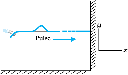
Fig. 14.2 When a pulse travels along the length of a stretched string (x-direction), the elements of the string oscillate up and down (y-direction)
Fig. 14.3 shows a similar situation, but this time the external agent gives a continuous periodic sinusoidal up and down jerk to one end of the string. The resulting disturbance on the string is then a sinusoidal wave. In either case the elements of the string oscillate about their equilibrium mean position as the pulse or wave passes through them. The oscillations are normal to the direction of wave motion along the string, so this is an example of transverse wave.
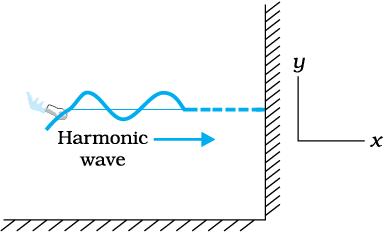
Fig. 14.3A harmonic (sinusoidal) wave travelling along a stretched string is an example of a transverse wave. An element of the string in the region of the wave oscillates about its equilibrium position perpendicular to the direction of wave propagation.
We can look at a wave in two ways. We can fix an instant of time and picture the wave in space. This will give us the shape of the wave as a whole in space at a given instant. Another way is to fix a location i.e. fix our attention on a particular element of string and see its oscillatory motion in time.
Fig. 14.4 describes the situation for longitudinal waves in the most familiar example of the propagation of sound waves. A long pipe filled with air has a piston at one end. A single sudden push forward and pull back of the piston will generate a pulse of condensations (higher density) and rarefactions (lower density) in the medium (air). If the push-pull of the piston is continuous and periodic (sinusoidal), a sinusoidal wave will be generated propagating in air along the length of the pipe. This is clearly an example of longitudinal waves.

The waves considered above, transverse or longitudinal, are travelling or progressive waves since they travel from one part of the medium to another. The material medium as a whole does not move, as already noted. A stream, for example, constitutes motion of water as a whole. In a water wave, it is the disturbance that moves, not water as a whole. Likewise a wind (motion of air as a whole) should not be confused with a sound wave which is a propagation of disturbance (in pressure density) in air, without the motion of air medium as a whole.
In transverse waves, the particle motion is normal to the direction of propagation of the wave. Therefore, as the wave propagates, each element of the medium undergoes a shearing strain. Transverse waves can, therefore, be propagated only in those media, which can sustain shearing stress, such as solids and not in fluids. Fluids, as well as, solids can sustain compressive strain; therefore, longitudinal waves can be propagated in all elastic media. For example, in medium like steel, both transverse and longitudinal waves can propagate, while air can sustain only longitudinal waves. The waves on the surface of water are of two kinds: capillary waves and gravity waves. The former are ripples of fairly short wavelength—not more than a few centimetre—and the restoring force that produces them is the surface tension of water. Gravity waves have wavelengths typically ranging from several metres to several hundred meters. The restoring force that produces these waves is the pull of gravity, which tends to keep the water surface at its lowest level. The oscillations of the particles in these waves are not confined to the surface only, but extend with diminishing amplitude to the very bottom. The particle motion in water waves involves a complicated motion—they not only move up and down but also back and forth. The waves in an ocean are the combination of both longitudinal and transverse waves.
It is found that, generally, transverse and longitudinal waves travel with different speed in the same medium.
Example 14.1 Given below are some examples of wave motion. State in each case if the wave motion is transverse, longitudinal or a combination of both:
(a) Motion of a kink in a longitudinal spring produced by displacing one end of the springsideways.
(b) Waves produced in a cylinder containing a liquid by moving its piston back and forth.
(c) Waves produced by a motorboat sailing in water.
(d) Ultrasonic waves in air produced by a vibrating quartz crystal.
Answer
(a) Transverse and longitudinal
(b) Longitudinal
(c) Transverse and longitudinal
(d) Longitudinal
14.3 Displacement relation in a progressive wave
For mathematical description of a travelling wave, we need a function of both position x and time t. Such a function at every instant should give the shape of the wave at that instant. Also, at every given location, it should describe the motion of the constituent of the medium at that location. If we wish to describe a sinusoidal travelling wave (such as the one shown in Fig. 14.3) the corresponding function must also be sinusoidal. For convenience, we shall take the wave to be transverse so that if the position of the constituents of the medium is denoted by x, the displacement from the equilibrium position may be denoted by y. A sinusoidal travelling wave is then described by:
 (14.2)
The term φ in the argument of sine function means equivalently that we are considering a linear combination of sine and cosine functions:
 (14.3)
From Equations (14.2) and (14.3),
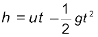
To understand why Equation (14.2) represents a sinusoidal travelling wave, take a fixed instant, say t = t0. Then, the argument of the sine function in Equation (14.2) is simply kx + constant. Thus, the shape of the wave (at any fixed instant) as a function of  is a sine wave. Similarly, take a fixed location, say x = x0. Then, the argument of the sine function in Equation (14.2) is constant -ωt. The displacement y, at a fixed location, thus, varies sinusoidally with time. That is, the constituents of the medium at different positions execute simple harmonic motion. Finally, as t increases, x must increase in the positive direction to keep kx – ωt + φ constant. Thus, Eq. (14.2) represents a sinusiodal (harmonic) wave travelling along the positive direction of the x-axis. On the other hand, a function
 (14.4)
represents a wave travelling in the negative direction of x-axis. Fig. (14.5) gives the names of the various physical quantities appearing in Eq. (14.2) that we now interpret.
y(x,t) : displacement as a function of position x and time t
a : amplitude of a wave
ω :angular frequency of the wave
k :angular wave number
kx–ωt+φ : initial phase angle (a+x = 0, t = 0)
Fig. 14.6 shows the plots of Eq. (14.2) for different values of time differing by equal intervals of time. In a wave, the crest is the point of maximum positive displacement, the trough is the point of maximum negative displacement. To see how a wave travels, we can fix attention on a crest and see how it progresses with time. In the figure, this is shown by a cross (×) on the crest. In the same manner, we can see the motion of a particular constituent of the medium at a fixed location, say at the origin of the x-axis. This is shown by a solid dot (•). The plots of Fig. 14.6 show that with time, the solid dot (•) at the origin moves periodically, i.e., the particle at the origin oscillates about its mean position as the wave progresses. This is true for any other location also. We also see that during the time the solid dot (•) has completed one full oscillation, the crest has moved further by a certain distance.
Fig. 14.6 A harmonic wave progressing along the positive direction of x-axis at different times.
Using the plots of Fig. 14.6, we now define the various quantities of Eq. (14.2).
14.3.1 Amplitude and Phase
In Eq. (14.2), since the sine function varies between 1 and –1, the displacement y (x,t) varies between a and –a. We can take a to be a positive constant, without any loss of generality. Then, a represents the maximum displacement of the constituents of the medium from their equilibrium position. Note that the displacement y may be positive or negative, but a is positive. It is called the amplitude of the wave.
The quantity (kx – ωt + φ) appearing as the argument of the sine function in Eq. (14.2) is called the phase of the wave. Given the amplitude a, the phase determines the displacement of the wave at any position and at any instant. Clearly φ is the phase at x = 0 and t = 0. Hence, φ is called the initial phase angle. By suitable choice of origin on the x-axis and the intial time, it is possible to have φ = 0. Thus there is no loss of generality in dropping φ, i.e., in taking Eq. (14.2) with φ = 0.
14.3.2 Wavelength and Angular Wave Number
The minimum distance between two points having the same phase is called the wavelength of the wave, usually denoted by λ. For simplicity, we can choose points of the same phase to be crests or troughs. The wavelength is then the distance between two consecutive crests or troughs in a wave. Taking φ = 0 in Eq. (14.2), the displacement at t = 0 is given by
 (14.5)
Since the sine function repeats its value after every 2π change in angle,
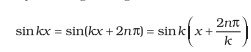
That is the displacements at points x and at

are the same, where n=1,2,3,... The 1east distance between points with the same displacement (at any given instant of time) is obtained by taking n = 1.  is then given by
 or
or  (14.6)
k is the angular wave number or propagation constant; its SI unit is radian per metre or  *
*
14.3.3 Period, Angular Frequency and Frequency
Fig. 14.7 shows again a sinusoidal plot. It describes not the shape of the wave at a certain instant but the displacement of an element (at any fixed location) of the medium as a function of time. We may for, simplicity, take Eq. (14.2) with φ = 0 and monitor the motion of the element say at  . We then get
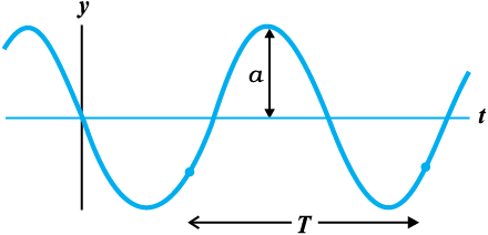
Fig. 14.7 An element of a string at a fixed location oscillates in time with amplitude a and period T, as the wave passes over it.
Now, the period of oscillation of the wave is the time it takes for an element to complete one full oscillation. That is

Since sine function repeats after every  ,
,
 or
or  (14.7)
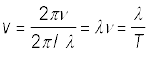
 is called the angular frequency of the wave. Its SI unit is rad s –1. The frequency ν is the number of oscillations per second. Therefore,
 (14.8)
 is usually measured in hertz.
In the discussion above, reference has always been made to a wave travelling along a string or a transverse wave. In a longitudinal wave, the displacement of an element of the medium is parallel to the direction of propagation of the wave. In Eq. (14.2), the displacement function for a longitudinal wave is written as,
s(x, t) = a sin (kx – ωt + φ) (14.9)
where s(x, t) is the displacement of an element of the medium in the direction of propagation of the wave at position x and time t. In Eq. (14.9), a is the displacement amplitude; other quantities have the same meaning as in case of a transverse wave except that the displacement function y (x, t) is to be replaced by the function s (x, t).
________________________________________
Example 14.2 A wave travelling along a string is described by,
y(x, t) = 0.005 sin (80.0 x – 3.0 t), in which the numerical constants are in SI units (0.005 m, 80.0 rad m–1, and 3.0 rad s–1). Calculate (a) the amplitude, (b) the wavelength, and (c) the period and frequency of the wave. Also, calculate the displacement y of the wave at a distance x = 30.0 cm and time t = 20 s ?
Answer On comparing this displacement equation with Eq. (14.2),
y (x, t) = a sin (kx – ωt),
we find
(a) the amplitude of the wave is 0.005 m = 5 mm.
(b) the angular wave number k and angular frequency ω are
k = 80.0 m–1 and ω = 3.0 s–1
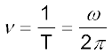
We, then, relate the wavelength λ to k through Eq. (14.6),
λ = 2π/k
= 7.85 cm
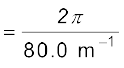
(c) Now, we relate T to ω by the relation
T = 2π/ω
= 2.09 s
and frequency, v = 1/T = 0.48 Hz
The displacement y at x = 30.0 cm and
time t = 20 s is given by
y = (0.005 m) sin (80.0 × 0.3 – 3.0 × 20)
= (0.005 m) sin (–36 + 12π)
= (0.005 m) sin (1.699)
= (0.005 m) sin (970) j 5 mm
14.4 The speed of a travelling wave
To determine the speed of propagation of a travelling wave, we can fix our attention on any particular point on the wave (characterised by some value of the phase) and see how that point moves in time. It is convenient to look at the motion of the crest of the wave. Fig. 14.8 gives the shape of the wave at two instants of time, which differ by a small time internal ∆t. The entire wave pattern is seen to shift to the right (positive direction of x-axis) by a distance ∆x. In particular, the crest shown by a dot ( ) moves a
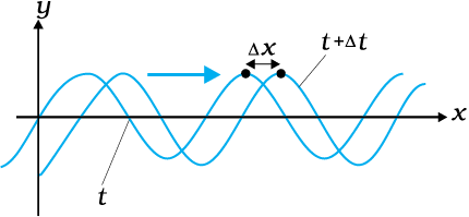
Fig. 14.8 Progression of a harmonic wave from time t to t + ∆t. where ∆t is a small interval. The wave pattern as a whole shifts to the right. The crest of the wave (or a point with any fixed phase) moves right by the distance ∆x in time ∆t.
distance ∆x in time ∆t. The speed of the wave is then ∆x/∆t. We can put the dot (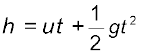 ) on a point with any other phase. It will move with the same speed v (otherwise the wave pattern will not remain fixed). The motion of a fixed phase point on the wave is given by
kx – ωt = constant (14.10)
Thus, as time t changes, the position x of the fixed phase point must change so that the phase remains constant. Thus,
kx – ωt = k(x+∆x) – ω(t+∆t)
or k ∆x – ω ∆t =0
Taking ∆x, ∆t vanishingly small, this gives
 (14.11)
Relating ω to T and k to λ, we get
 (14.12)
Eq. (14.12), a general relation for all progressive waves, shows that in the time required for one full oscillation by any constituent of the medium, the wave pattern travels a distance equal to the wavelength of the wave. It should be noted that the speed of a mechanical wave is determined by the inertial (linear mass density for strings, mass density in general) and elastic properties (Young’s modulus for linear media/ shear modulus, bulk modulus) of the medium. The medium determines the speed; Eq. (14.12) then relates wavelength to frequency for the given speed. Of course, as remarked earlier, the medium can support both transverse and longitudinal waves, which will have different speeds in the same medium. Later in this chapter, we shall obtain specific expressions for the speed of mechanical waves in some media.
14.4.1 Speed of a Transverse Wave on Stretched String
The speed of a mechanical wave is determined by the restoring force setup in the medium when it is disturbed and the inertial properties (mass density) of the medium. The speed is expected to be directly related to the former and inversely to the latter. For waves on a string, the restoring force is provided by the tension T in the string. The inertial property will in this case be linear mass density µ, which is mass m of the string divided by its length L. Using Newton’s Laws of Motion, an exact formula for the wave speed on a string can be derived, but this derivation is outside the scope of this book. We shall, therefore, use dimensional analysis. We already know that dimensional analysis alone can never yield the exact formula. The overall dimensionless constant is always left undetermined by dimensional analysis.
The dimension of µ is [ML-1] and that of T is like force, namely [MLT-2]. We need to combine these dimensions to get the dimension of speed v [LT-1]. Simple inspection shows that the quantity T/µ has the relevant dimension
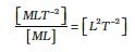
Thus if T and µ are assumed to be the only relevant physical quantities,
v = C  (14.13)
where C is the undetermined constant of dimensional analysis. In the exact formula, it turms out, C=1. The speed of transverse waves on a stretched string is given by
v =  (14.14)
Note the important point that the speed v depends only on the properties of the medium T and µ (T is a property of the stretched string arising due to an external force). It does not depend on wavelength or frequency of the wave itself. In higher studies, you will come across waves whose speed is not independent of frequency of the wave. Of the two parameters λ and ν the source of disturbance determines the frequency of the wave generated. Given the speed of the wave in the medium and the frequency Eq. (14.12) then fixes the wavelength
 (14.15)
Example 14.3 A steel wire 0.72 m long has a mass of 5.0 ×10⁻³ kg. If the wire is under a tension of 60 N, what is the speed of transverse waves on the wire ?
Answer Mass per unit length of the wire,
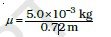
= 6.9 ×10⁻³ kg m–1
Tension, T = 60 N
The speed of wave on the wire is given by
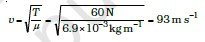
14.4.2 Speed of a Longitudinal Wave (Speed of Sound)
In a longitudinal wave, the constituents of the medium oscillate forward and backward in the direction of propagation of the wave. We have already seen that the sound waves travel in the form of compressions and rarefactions of small volume elements of air. The elastic property that determines the stress under compressional strain is the bulk modulus of the medium defined by (see Chapter 8)
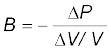 (14.16)
Here, the change in pressure ∆P produces a volumetric strain  . B has the same dimension as pressure and given in SI units in terms of pascal (Pa). The inertial property relevant for the propagation of wave is the mass density ρ, with dimensions [ML-3]. Simple inspection reveals that quantity B/ρ has the relevant dimension:
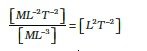 (14.17)
Thus, if B and  are considered to be the only relevant physical quantities,
v = C  (14.18)
where, as before, C is the undetermined constant from dimensional analysis. The exact derivation shows that C=1. Thus, the general formula for longitudinal waves in a medium is:
v =  (14.19)
For a linear medium, like a solid bar, the lateral expansion of the bar is negligible and we may consider it to be only under longitudinal strain. In that case, the relevant modulus of elasticity is Young’s modulus, which has the same dimension as the Bulk modulus. Dimensional analysis for this case is the same as before and yields a relation like Eq. (14.18), with an undetermined C, which the exact derivation shows to be unity. Thus, the speed of longitudinal waves in a solid bar is given by
v =  (14.20)
where Y is the Young’s modulus of the material of the bar. Table 14.1 gives the speed of sound in some media.
Table 14.1 Speed of Sound in some Media
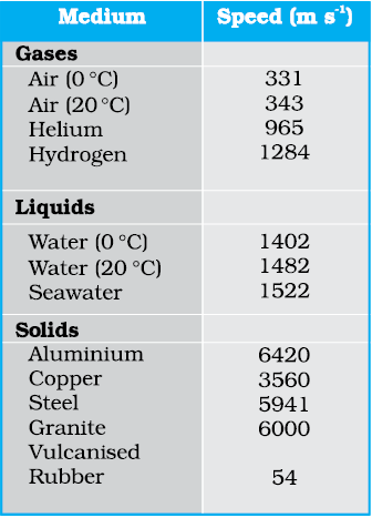
Liquids and solids generally have higher speed of sound than gases. [Note for solids, the speed being referred to is the speed of longitudinal waves in the solid]. This happens because they are much more difficult to compress than gases and so have much higher values of bulk modulus. Now, see Eq. (14.19). Solids and liquids have higher mass densities ( ) than gases. But the corresponding increase in both the modulus (B) of solids and liquids is much higher. This is the reason why the sound waves travel faster in solids and liquids.
We can estimate the speed of sound in a gas in the ideal gas approximation. For an ideal gas, the pressure P, volume V and temperature T are related by (see Chapter 10).
PV = NkBT (14.21)
where N is the number of molecules in volume V, kB is the Boltzmann constant and T the temperature of the gas (in Kelvin). Therefore, for an isothermal change it follows from Eq.(14.21) that
V∆P + P∆V = 0
or 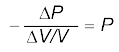
Hence, substituting in Eq. (14.16), we have
B = P
Therefore, from Eq. (14.19) the speed of a longitudinal wave in an ideal gas is given by,
v =  (14.22)
This relation was first given by Newton and is known as Newton’s formula.
Example 14.4 Estimate the speed of sound in air at standard temperature and pressure. The mass of 1 mole of air is 29.0×10⁻³ kg.
Answer We know that 1 mole of any gas occupies 22.4 litres at STP. Therefore, density of air at STP is:
ρo = (mass of one mole of air)/ (volume of one
mole of air at STP)
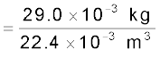
= 1.29 kg m–3
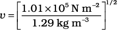 = 280 m s–1 (14.23)
The result shown in Eq.(14.23) is about 15% smaller as compared to the experimental value of 331 m s–1 as given in Table 14.1.Where did we go wrong? If we examine the basic assumption made by Newton that the pressure variations in a medium during propagation of sound are isothermal, we find that this is not correct. It was pointed out by Laplace that the pressure variations in the propagation of sound waves are so fast that there is little time for the heat flow to maintain constant temperature. These variations, therefore, are adiabatic and not isothermal. For adiabatic processes the ideal gas satisfies the relation (see Section 11.8),
PVγ = constant
i.e. ∆(PVγ ) = 0
or Pγ V γ –1 ∆V + Vγ ∆P = 0
where γ is the ratio of two specific heats,
Cp/Cv.
Thus, for an ideal gas the adiabatic bulk modulus is given by,
Bad = 
= γP
The speed of sound is, therefore, from Eq. (14.19), givenby,
v =  (14.24)
This modification of Newton’s formula is referred to as the Laplace correction. For air γ = 7/5. Now using Eq. (14.24) to estimate the speed of sound in air at STP, we get a value 331.3 m s–1, which agrees with the measured speed.
14.5 The principle of superposition of waves
What happens when two wave pulses travelling in opposite directions cross each other
(Fig. 14.9)? It turns out that wave pulses continue to retain their identities after they have crossed. However, during the time they overlap, the wave pattern is different from either of the pulses. Figure 14.9 shows the situation when two pulses of equal and opposite shapes move towards each other. When the pulses overlap, the resultant displacement is the algebraic sum of the displacement due to each pulse. This is known as the principle of superposition of waves.
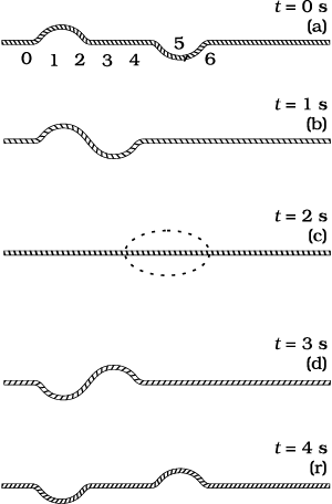
Fig. 14.9 Two pulses having equal and opposite displacements moving in opposite directions. The overlapping pulses add up to zero displacement in curve (c).
According to this principle, each pulse moves as if others are not present. The constituents of the medium, therefore, suffer displacments due to both and since the displacements can be positive and negative, the net displacement is an algebraic sum of the two. Fig. 14.9 gives graphs of the wave shape at different times. Note the dramatic effect in the graph (c); the displacements due to the two pulses have exactly cancelled each other and there is zero displacement throughout.
To put the principle of superposition mathematically, let y1 (x,t) and y2 (x,t) be the displacements due to two wave disturbances in the medium. If the waves arrive in a region simultaneously, and therefore, overlap, the net displacement y (x,t) is given by
y (x, t) = y1(x, t) + y2(x, t) (14.25)
If we have two or more waves moving in the medium the resultant waveform is the sum of wave functions of individual waves. That is, if the wave functions of the moving waves are
y1 = f1(x–vt),
y2 = f2(x–vt),
..........
..........
yn = fn (x–vt)
then the wave function describing the disturbance in the medium is
y = f1(x – vt)+ f2(x – vt)+ ...+ fn(x – vt)
 (14.26)
The principle of superposition is basic to the phenomenon of interference.
For simplicity, consider two harmonic travelling waves on a stretched string, both with the same ω (angular frequency) and k (wave number), and, therefore, the same wavelength λ. Their wave speed will be identical. Let us further assume that their amplitudes are equal and they are both travelling in the positive direction of x-axis. The waves only differ in their initial phase. According to Eq. (14.2), the two waves are described by the functions:
y1(x, t) = a sin (kx – ωt) (14.27)
and y2(x, t) = a sin (kx – ωt + φ ) (14.28)
The net displacement is then, by the principle of superposition, given by
y (x, t) = a sin (kx – ωt) + a sin (kx – ωt + φ) (14.29)
 (14.30)
where we have used the familiar trignometric identity for