
Chapter 6
Open Economy Macroeconomics
An open economy is one which interacts with other countries through various channels. So far we had not considered this aspect and just limited to a closed economy in which there are no linkages with the rest of the world in order to simplify our analysis and explain the basic macroeconomic mechanisms. In reality, most modern economies are open.
There are three ways in which these linkages are established.
1. Output Market: An economy can trade in goods and services with other countries. This widens choice in the sense that consumers and producers can choose between domestic and foreign goods.
2. Financial Market: Most often an economy can buy financial assets from other countries. This gives investors the opportunity to choose between domestic and foreign assets.
3. Labour Market: Firms can choose where to locate production and workers to choose where to work. There are various immigration laws which restrict the movement of labour between countries.
Movement of goods has traditionally been seen as a substitute for the movement of labour. We focus on the first two linkages. Thus, an open economy is said to be one that trades with other nations in goods and services and most often, also in financial assets. Indians for instance, can consume products which are produced around the world and some of the products from India are exported to other countries.
Foreign trade, therefore, influences Indian aggregate demand in two ways. First, when Indians buy foreign goods, this spending escapes as a leakage from the circular flow of income decreasing aggregate demand. Second, our exports to foreigners enter as an injection into the circular flow, increasing aggregate demand for goods produced within the domestic economy.
When goods move across national borders, money must be used for the transactions. At the international level there is no single currency that is issued by a single bank. Foreign economic agents will accept a national currency only if they are convinced that the amount of goods they can buy with a certain amount of that currency will not change frequently. In other words, the currency will maintain a stable purchasing power. Without this confidence, a currency will not be used as an international medium of exchange and unit of account since there is no international authority with the power to force the use of a particular currency in international transactions.
In the past, governments have tried to gain confidence of potential users by announcing that the national currency will be freely convertible at a fixed price into another asset. Also, the issuing authority will have no control over the value of that asset into which the currency can be converted. This other asset most often has been gold, or other national currencies. There are two aspects of this commitment that has affected its credibility — the ability to convert freely in unlimited amounts and the price at which this conversion takes place. The international monetary system has been set up to handle these issues and ensure stability in international transactions.
With the increase in the volume of transactions, gold ceased to be the asset into which national currencies could be converted (See Box 6.2). Although some national currencies have international acceptability, what is important in transactions between two countries is the currency in which the trade occurs. For instance, if an Indian wants to buy a good made in America, she would need dollars to complete the transaction. If the price of the good is ten dollars, she would need to know how much it would cost her in Indian rupees. That is, she will need to know the price of dollar in terms of rupees. The price of one currency in terms of another currency is known as the foreign exchange rate or simply the exchange rate. We will discuss this in detail in section 6.2.
6.1 The Balance of Payments
The balance of payments (BoP) record the transactions in goods, services and assets between residents of a country with the rest of the world for a specified time period typically a year. There are two main accounts in the BoP — the current account and the capital account1.
6.1.1 Current Account
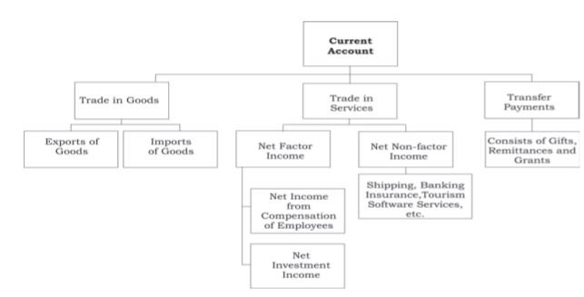
Current Account is the record of trade in goods and services and transfer payments. Figure 6.1 illustrates the components of Current Account. Trade in goods includes exports and imports of goods. Trade in services includes factor income and non-factor income transactions. Transfer payments are the receipts which the residents of a country get for ‘free’, without having to provide any goods or services in return. They consist of gifts, remittances and grants. They could be given by the government or by private citizens living abroad.
Buying foreign goods is expenditure from our country and it becomes the income of that foreign country. Hence, the purchase of foreign goods or imports decreases the domestic demand for goods and services in our country. Similarly, selling of foreign goods or exports brings income to our country and adds to the aggregate domestic demand for goods and services in our country.
1 There is a new classification in which the balance of payments have been divided into three
accounts — the current account, the financial account and the capital account. This is as per the
new accounting standards specified by the International Monetary Fund (IMF) in the sixth edition of
the Balance of Payments and International Investment Position Manual (BPM6). India has also
made the change but the Reserve Bank of India continues to publish data accounting to the old
classification.
Fig. 6.1: Components of Current Account
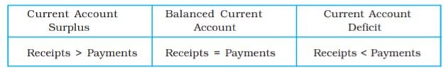
Balance on Current Account
Current Account is in balance when receipts on current account are equal to the payments on the current account. A surplus current account means that the nation is a lender to other countries and a deficit current account means that the nation is a borrower from other countries.
Balance on Current Account has two components:
• ·Balance of Trade or Trade Balance
• ·Balance on Invisibles
Balance of Trade (BOT) is the difference between the value of exports and value of imports of goods of a country in a given period of time. Export of goods is entered as a credit item in BOT, whereas import of goods is entered as a debit item in BOT. It is also known as Trade Balance.
BOT is said to be in balance when exports of goods are equal to the imports of goods. Surplus BOT or Trade surplus will arise if country exports more goods than what it imports. Whereas, Deficit BOT or Trade deficit will arise if a country imports more goods than what it exports.
Net Invisibles is the difference between the value of exports and value of imports of invisibles of a country in a given period of time. Invisibles include services, transfers and flows of income that take place between different countries. Services trade includes both factor and non-factor income. Factor income includes net international earnings on factors of production (like labour, land and capital). Non-factor income is net sale of service products like shipping, banking, tourism, software services, etc.
6.1.2 Capital Account
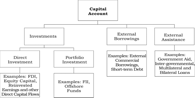
Capital Account records all international transactions of assets. An asset is any one of the forms in which wealth can be held, for example: money, stocks, bonds, Government debt, etc. Purchase of assets is a debit item on the capital account. If an Indian buys a UK Car Company, it enters capital account transactions as a debit item (as foreign exchange is flowing out of India). On the other hand, sale of assets like sale of share of an Indian company to a Chinese customer is a credit item on the capital account. Fig. 6.2 classifies the items which are a part of capital account transactions. These items are Foreign Direct Investments (FDIs), Foreign Institutional Investments (FIIs), external borrowings and assistance.
Fig. 6.2: Components of Capital Account
Balance on Capital Account
Capital account is in balance when capital inflows (like receipt of loans from abroad, sale of assets or shares in foreign companies) are equal to capital outflows (like repayment of loans, purchase of assets or shares in foreign countries). Surplus in capital account arises when capital inflows are greater than capital outflows, whereas deficit in capital account arises when capital inflows are lesser than capital outflows.
6.1.3 Balance of Payments Surplus and Deficit
The essence of international payments is that just like an individual who spends more than her income must finance the difference by selling assets or by borrowing, a country that has a deficit in its current account (spending more than it receives from sales to the rest of the world) must finance it by selling assets or by borrowing abroad. Thus, any current account deficit must be financed by a capital account surplus, that is, a net capital inflow.
![]()
In this case, in which a country is said to be in balance of payments equilibrium, the current account deficit is financed entirely by international lending without any reserve movements.
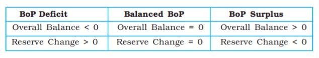
Alternatively, the country could use its reserves of foreign exchange in order to balance any deficit in its balance of payments. The reserve bank sells foreign exchange when there is a deficit. This is called official reserve sale. The decrease (increase) in official reserves is called the overall balance of payments deficit (surplus). The basic premise is that the monetary authorities are the ultimate financiers of any deficit in the balance of payments (or the recipients of any surplus).
We note that official reserve transactions are more relevant under a regime of fixed exchange rates than when exchange rates are floating. (See sub heading ‘Fixed Exchange Rates’ under section 6.2.2)
Autonomous and Accommodating Transactions
International economic transactions are called autonomous when transactions are made due to some reason other than to bridge the gap in the balance of payments, that is, when they are independent of the state of BoP. One reason could be to earn profit. These items are called ‘above the line’ items in the BoP. The balance of payments is said to be in surplus (deficit) if autonomous receipts are greater (less) than autonomous payments.
Accommodating transactions (termed ‘below the line’ items), on the other hand, are determined by the gap in the balance of payments, that is, whether there is a deficit or surplus in the balance of payments. In other words, they are determined by the net consequences of the autonomous transactions. Since the official reserve transactions are made to bridge the gap in the BoP, they are seen as the accommodating item in the BoP (all others being autonomous).
Errors and Omissions
It is difficult to record all international transactions accurately. Thus, we have a third element of BoP (apart from the current and capital accounts) called errors and omissions which reflects this.
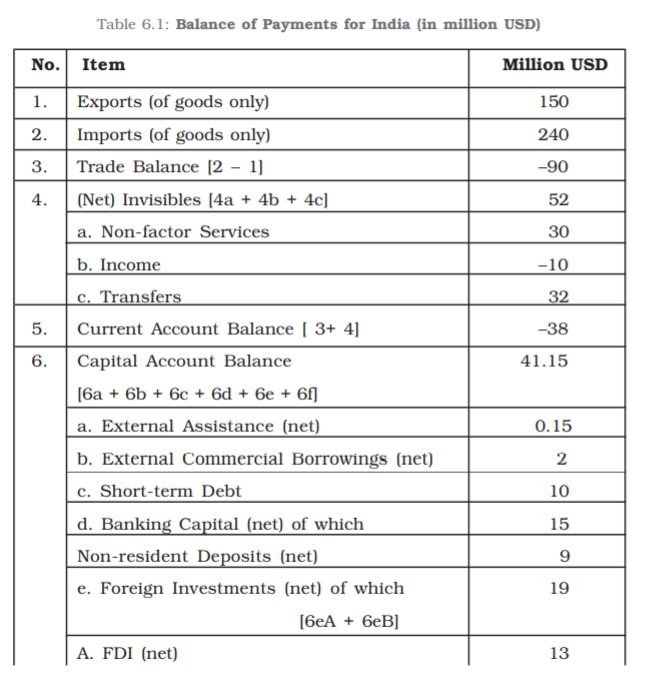
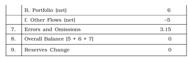
Table 6.1 provides a sample of Balance of Payments for India.
Note in this table, there is a trade deficit and current account deficit but a capital account surplus. As a result, BOP is in balance.
Box 6.1: The balance of payments accounts presented above divide the transactions into two accounts, current account and capital account. However, following the new accounting standards introduced by the International Monetary Fund in the sixth edition of the Balance of Payments and International Investment Position Manual (BPM6) the Reserve Bank of India also made changes in the structure of balance of payments accounts. According to the new classification, the transactions are divided into three accounts: current account, financial account and capital account. The most important change is that almost all the transactions arising on account of trade in financial assets such as bonds and equity shares are now placed in the financial account. However, RBI continues to publish the balance of payments accounts as per the old system also, therefore the details of the new system are not being given here. The details are given in the Balance of Payments Manual for India published by the Reserve Bank of India in September 2010.
Table 6.1: Balance of Payments for India (in million USD)
6.2 The Foreign Exchange Market
So far, we have considered the accounting of international transactions on the whole, we will now take up a single transaction. Let us assume that a single Indian resident wants to visit London on a vacation (an import of tourist services). She will have to pay in pounds for her stay there. She will need to know where to obtain the pounds and at what price. As mentioned at the beginning of this chapter, this price is known as the exchange rate. The market in which national currencies are traded for one another is known as the foreign exchange market.
The major participants in the foreign exchange market are commercial banks, foreign exchange brokers and other authorised dealers and monetary authorities. It is important to note that although participants themselves may have their own trading centres , the market itself is world-wide. There is a close and continuous contact between the trading centres and the participants deal in more than one market.
6.2.1 Foreign Exchange Rate
Foreign Exchange Rate (also called Forex Rate) is the price of one currency in terms of another. It links the currencies of different countries and enables comparison of international costs and prices. For example, if we have to pay Rs 50 for $1 then the exchange rate is Rs 50 per dollar.
To make it simple, let us consider that India and USA are the only countries in the world and so there is only one exchange rate that needs to be determined.
Demand for Foreign Exchange
People demand foreign exchange because: they want to purchase goods and services from other countries; they want to send gifts abroad; and, they want to purchase financial assets of a certain country.
A rise in price of foreign exchange will increase the cost (in terms of rupees) of purchasing a foreign good. This reduces demand for imports and hence demand for foreign exchange also decreases, other things remaining constant.
Supply of Foreign Exchange
Foreign currency flows into the home country due to the following reasons: exports by a country lead to the purchase of its domestic goods and services by the foreigners; foreigners send gifts or make transfers; and, the assets of a home country are bought by the foreigners.
A rise in price of foreign exchange will reduce the foreigner’s cost (in terms of USD) while purchasing products from India, other things remaining constant. This increases India’s exports and hence supply for foreign exchange may increase (whether it actually increases depends on a number of factors, particularly elasticity of demand for exports and imports.
6.2.2 Determination of the Exchange Rate
Different countries have different methods of determining their currency’s exchange rate. It can be determined through Flexible Exchange Rate, Fixed Exchange Rate or Managed Floating Exchange Rate.
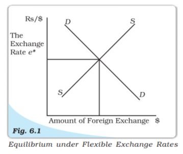
Flexible Exchange Rate
This exchange rate is determined by the market forces of demand and supply. It is also known as Floating Exchange Rate. As depicted in Fig. 6.1, the exchange rate is determined where the demand curve intersects with the supply curve, i.e., at point e on the Y – axis. Point q on the x – axis determines the quantity of US Dollars that have been demanded and supplied on e exchange rate. In a completely flexible system, the Central banks do not intervene in the foreign exchange market.
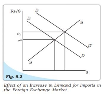
Suppose the demand for foreign goods and services increases (for example, due to increased international travelling by Indians), then as depicted in Fig. 6.2, the demand curve shifts upward and right to the original demand curve. The increase in demand for foreign goods and services result in a change in the exchange rate. The initial exchange rate e0 = 50, which means that we need to exchange Rs 50 for one dollar. At the new equilibrium, the exchange rate becomes e1 = 70, which means that we need to pay more rupees for a dollar now (i.e., Rs 70). It indicates that the value of rupees in terms of dollars has fallen and value of dollar in terms of rupees has risen. Increase in exchange rate implies that the price of foreign currency (dollar) in terms of domestic currency (rupees) has increased. This is called Depreciation of domestic currency (rupees) in terms of foreign currency (dollars).
Similarly, in a flexible exchange rate regime, when the price of domestic currency (rupees) in terms of foreign currency (dollars) increases, it is called Appreciation of the domestic currency (rupees) in terms of foreign currency (dollars). This means that the value of rupees relative to dollar has risen and we need to pay fewer rupees in exchange for one dollar.
Speculation
Money in any country is an asset. If Indians believe that British pound is going to increase in value relative to the rupee, they will want to hold pounds. Thus exchange rates also get affected when people hold foreign exchange on the expectation that they can make gains from the appreciation of the currency. This expectation in turn can actually affect the exchange rate in the following way. If the current exchange rate is Rs. 80 to a pound and investors believe that the pound is going to appreciate by the end of the month and will be worth Rs.85, investors think if they gave the dealer Rs. 80,000 and bought 1000 pounds, at the end of the month, they would be able to exchange the pounds for Rs. 85,000, thus making a profit of Rs. 5,000. This expectation would increase the demand for pounds and cause the rupee-pound exchange rate to increase in the present, making the beliefs self-fulfilling.
Interest Rates and the Exchange Rate
In the short run, another factor that is important in determining exchange rate movements is the interest rate differential i.e. the difference between interest rates between countries. There are huge funds owned by banks, multinational corporations and wealthy individuals which move around the world in search of the highest interest rates. If we assume that government bonds in country A pay 8 per cent rate of interest whereas equally safe bonds in county B yield 10 per cent, the interest rate differential is 2 per cent. Investors from country A will be attracted by the high interest rates in country B and will buy the currency of country B selling their own currency. At the same time investors in country B will also find investing in their own country more attractive and will therefore demand less of country A’s currency. This means that the demand curve for country A’s currency will shift to the left and the supply curve will shift to the right causing a depreciation of country A’s currency and an appreciation of country B’s currency. Thus, a rise in the interest rates at home often leads to an appreciation of the domestic currency. Here, the implicit assumption is that no restrictions exist in buying bonds issued by foreign governments.
Income and the Exchange Rate
When income increases, consumer spending increases. Spending on imported goods is also likely to increase. When imports increase, the demand curve for foreign exchange shifts to the right. There is a depreciation of the domestic currency. If there is an increase in income abroad as well, domestic exports will rise and the supply curve of foreign exchange shifts outward. On balance, the domestic currency may or may not depreciate. What happens will depend on whether exports are growing faster than imports. In general, other things remaining equal, a country whose aggregate demand grows faster than the rest of the world’s normally finds its currency depreciating because its imports grow faster than its exports. Its demand curve for foreign currency shifts faster than its supply curve
Exchange Rates in the Long Run
The purchasing Power (PPP) theory is used to make long-run predictions about exchange rates in a flexible exchange rate system. According to the theory, as long as there are no barriers to trade like tariffs (taxes on trade) and quotas (quantitative limits on imports), exchange rates should eventually adjust so that the same product costs the same whether measured in rupees in India, or dollars in the US, yen in Japan and so on, except for differences in transportation. Over the long run, therefore, exchange rates between any two national currencies adjust to reflect differences in the price levels in the two countries.
EXAMPLE ![]() 6.1
6.1
If a shirt costs $8 in the US and Rs 400 in India, the rupee-dollar exchange rate should be Rs 50. To see why, at any rate higher than Rs 50, say Rs 60, it costs Rs 480 per shirt in the US but only Rs 400 in India. In that case, all foreign customers would buy shirts from India. Similarly, any exchange rate below Rs 50 per dollar will send all the shirt business to the US. Next, we suppose that prices in India rise by 20 per cent while prices in the US rise by 50 per cent. Indian shirts would now cost Rs 480 per shirt while American shirts cost $12 per shirt. For these two prices to be equivalent, $12 must be worth Rs 480, or one dollar must be worth Rs 40. The dollar, therefore, has depreciated.
Fixed Exchange Rates
In this exchange rate system, the Government fixes the exchange rate at a particular level. In Fig. 6.3, the market determined exchange rate is e. However, let us suppose that for some reason the Indian Government wants to encourage exports for which it needs to make rupee cheaper for foreigners it would do so by fixing a higher exchange rate, say Rs 70 per dollar from the current exchange rate of Rs 50 per dollar. Thus, the new exchange rate set by the Government is e1, where e1 > e. At this exchange rate, the supply of dollars exceeds the demand for dollars. The RBI intervenes to purchase the dollars for rupees in the foreign exchange market in order to absorb this excess supply which has been marked as AB in the figure. Thus, through intervention, the Government can maintain any exchange rate in the economy. But it will be accumulating more and more foreign exchange so long as this intervention goes on. On the other hand if the goverment was to set an exchange rate at a level such as e2, there would be an excess demand for dollars in the foreign exchange market. To meet this excess demand for dollars, the government would have to withdraw dollars from its past holdings of dollars. If it fails to do so, a black market for dollars may come up.
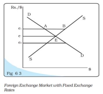
In a fixed exchange rate system, when some government action increases the exchange rate (thereby, making domestic currency cheaper) is called Devaluation. On the other hand, a Revaluation is said to occur, when the Government decreases the exchange rate (thereby, making domestic currency costlier) in a fixed exchange rate system.
6.2.3 Merits and Demerits of Flexible and Fixed Exchange Rate Systems
The main feature of the fixed exchange rate system is that there must be credibility that the government will be able to maintain the exchange rate at the level specified. Often, if there is a deficit in the BoP, in a fixed exchange rate system, governments will have to intervene to take care of the gap by use of its official reserves. If people know that the amount of reserves is inadequate, they would begin to doubt the ability of the government to maintain the fixed rate. This may give rise to speculation of devaluation. When this belief translates into aggressive buying of one currency thereby forcing the government to devalue, it is said to constitute a speculative attack on a currency. Fixed exchange rates are prone to these kinds of attacks, as has been witnessed in the period before the collapse of the Bretton Woods System.
The flexible exchange rate system gives the government more flexibility and they do not need to maintain large stocks of foreign exchange reserves. The major advantage of flexible exchange rates is that movements in the exchange rate automatically take care of the surpluses and deficits in the BoP. Also, countries gain independence in conducting their monetary policies, since they do not have to intervene to maintain exchange rate which are automatically taken care of by the market.
6.2.4 Managed Floating
Without any formal international agreement, the world has moved on to what can be best described as a managed floating exchange rate system. It is a mixture of a flexible exchange rate system (the float part) and a fixed rate system (the managed part). Under this system, also called dirty floating, central banks intervene to buy and sell foreign currencies in an attempt to moderate exchange rate movements whenever they feel that such actions are appropriate. Official reserve transactions are, therefore, not equal to zero.
Box 6.2 Exchange Rate Management: The International Experience
The Gold Standard: From around 1870 to the outbreak of the First World War in 1914, the prevailing system was the gold standard which was the epitome of the fixed exchange rate system. All currencies were defined in terms of gold; indeed some were actually made of gold. Each participant country committed to guarantee the free convertibility of its currency into gold at a fixed price. This meant that residents had, at their disposal, a domestic currency which was freely convertible at a fixed price into another asset (gold) acceptable in international payments. This also made it possible for each currency to be convertible into all others at a fixed price. Exchange rates were determined by its worth in terms of gold (where the currency was made of gold, its actual gold content). For example, if one unit of say currency A was worth one gram of gold, one unit of currency B was worth two grams of gold, currency B would be worth twice as much as currency A. Economic agents could directly convert one unit of currency B into two units of currency A, without having to first buy gold and then sell it. The rates would fluctuate between an upper and a lower limit, these limits being set by the costs of melting, shipping and recoining between the two Currencies3. To maintain the official parity each country needed an adequate stock of gold reserves. All countries on the gold standard had stable exchange rates.
The question arose – would not a country lose all its stock of gold if it imported too much (and had a BoP deficit)? The mercantilist4 explanation was that unless the state intervened, through tariffs or quotas or subsidies, on exports, a country would lose its gold and that was considered one of the worst tragedies. David Hume, a noted philosopher writing in 1752, refuted this view and pointed out that if the stock of gold went down, all prices and costs would fall commensurately and no one in the country would be worse off. Also, with cheaper goods at home, imports would fall and exports rise (it is the real exchange rate which will determine competitiveness). The country from which we were importing and making payments in gold would face an increase in prices and costs, so their now expensive exports would fall and their imports of the first country’s now cheap goods would go up. The result of this price-specie-flow (precious metals were referred to as ‘specie’ in the eighteenth century) mechanism is normally to improve the BoP of the country losing gold, and worsen that of the country with the favourable trade balance, until equilibrium in international trade is re-established at relative prices that keep imports and exports in balance with no further net gold flow. The equilibrium is stable and self-correcting, requiring no tariffs and state action. Thus, fixed exchange rates were maintained by an automatic equilibrating mechanism.
Several crises caused the gold standard to break down periodically. Moreover, world price levels were at the mercy of gold discoveries. This can be explained by looking at the crude Quantity Theory of Money, M = kPY, according to which, if output (GNP) increased at the rate of 4 per cent per year, the gold supply would have to increase by 4 per cent per year to keep prices stable. With mines not producing this much gold, price levels were falling all over the world in the late nineteenth century, giving rise to social unrest. For a period, silver supplemented gold introducing ‘bimetallism’. Also,fractional reserve banking helped to economise on gold. Paper currency was not entirely backed by gold; typically countries held one-fourth gold against its paper currency. Another way of economising on gold was the gold exchange standard which was adopted by many countries which kept their money exchangeable at fixed prices with respect to gold but held little or no gold. Instead of gold, they held the currency of some large country (the United States or the United Kingdom) which was on the gold standard. All these and the discovery of gold in Klondike and South Africa helped keep deflation at bay till 1929. Some economic historians attribute the Great Depression to this shortage of liquidity. During 1914-45, there was no maintained universal system but this period saw both a brief return to the gold standard and a period of flexible exchange rates.
The Bretton Woods System: The Bretton Woods Conference held in 1944 set up the International Monetary Fund (IMF) and the World Bank and reestablished a system of fixed exchange rates. This was different from the international gold standard in the choice of the asset in which national currencies would be convertible. A two-tier system of convertibility was established at the centre of which was the dollar. The US monetary authorities guaranteed the convertibility of the dollar into gold at the fixed price of $35 per ounce of gold. The second-tier of the system was the commitment of monetary authority of each IMF member participating in the system to convert their currency into dollars at a fixed price. The latter was called the official exchange rate. For instance, if French francs could be exchanged for dollars at roughly 5 francs per dollar, the dollars could then be exchanged for gold at $35 per ounce, which fixed the value of the franc at 175 francs per ounce of gold (5 francs per dollar times 35 dollars per ounce). A change in exchange rates was to be permitted only in case of a ‘fundamental disequilibrium’ in a nation’s BoP – which came to mean a chronic deficit in the BoP of sizeable proportions.
Such an elaborate system of convertibility was necessary because the distribution of gold reserves across countries was uneven with the US having almost 70 per cent of the official world gold reserves. Thus, a credible gold convertibility of the other currencies would have required a massive redistribution of the gold stock. Further, it was believed that the existing gold stock would be insufficient to sustain the growing demand for international liquidity. One way to save on gold, then, was a two-tier convertible system, where the key currency would be convertible into gold and the other currencies into the key currency.
In the post–World War II scenario, countries devastated by the war needed enormous resources for reconstruction. Imports went up and their deficits were financed by drawing down their reserves. At that time, the US dollar was the main component in the currency reserves of the rest of the world, and those reserves had been expanding as a consequence of the US running a continued balance of payments deficit (other countries were willing to hold those dollars as a reserve asset because they were committed to maintain convertibility between their currency and the dollar).
The problem was that if the short-run dollar liabilities of the US continued to increase in relation to its holdings of gold, then the belief in the credibility of the US commitment to convert dollars into gold at the fixed price would be eroded. The central banks would thus have an overwhelming incentive to convert the existing dollar holdings into gold, and that would, in turn, force the US to give up its commitment. This was the Triffin Dilemma after Robert Triffin, the main critic of the Bretton Woods system. Triffin suggested that the IMF should be turned into a ‘deposit bank’ for central banks and a new ‘reserve asset’ be created under the control of the IMF. In 1967, gold was displaced by creating the Special Drawing Rights (SDRs), also known as ‘paper gold’, in the IMF with the intention of increasing the stock of international reserves. Originally defined in terms of gold, with 35 SDRs being equal to one ounce of gold (the dollar-gold rate of the Bretton Woods system), it has been redefined several times since 1974. At present, it is calculated daily as the weighted sum of the values in dollars of four currencies (euro, dollar, Japanese yen, pound sterling) of the five countries (France, Germany, Japan, the UK and the US). It derives its strength from IMF members being willing to use it as a reserve currency and use it as a means of payment between central banks to exchange for national currencies. The original installments of SDRs were distributed to member countries according to their quota in the Fund (the quota was broadly related to the country’s economic importance as indicated by the value of its international trade).
The breakdown of the Bretton Woods system was preceded by many events, such as the devaluation of the pound in 1967, flight from dollars to gold in 1968 leading to the creation of a two-tiered gold market (with the official rate at $35 per ounce and the private rate market determined), and finally in August 1971, the British demand that US guarantee the gold value of its dollar holdings. This led to the US decision to give up the link between the dollar and gold: USA announced it would no longer be willing to convert dollars into gold at 35$ per ounce.
The ‘Smithsonian Agreement’ in 1971, which widened the permissible band of movements of the exchange rates to 2.5 per cent above or below the new ‘central rates’ with the hope of reducing pressure on deficit countries, lasted only 14 months. The developed market economies, led by the United Kingdom and soon followed by Switzerland and then Japan, began to adopt floating exchange rates in the early 1970s. In 1976, revision of IMF Articles allowed countries to choose whether to float their currencies or to peg them (to a single currency, a basket of currencies, or to the SDR). There are no rules governing pegged rates and no de facto supervision of floating exchange rates.
The Current Scenario: Many countries currently have fixed exchange rates. The creation of the European Monetary Union in January, 1999, involved permanently fixing the exchange rates between the currencies of the members of the Union and the introduction of a new common currency, the Euro, under the management of the European Central Bank. From January, 2002, actual notes and coins were introduced. So far, 12 of the 25 members of the European Union have adopted the euro.
Some countries pegged their currency to the French franc; most of these are former French colonies in Africa. Others peg to a basket of currencies, with the weights reflecting the composition of their trade. Often smaller countries also decide to fix their exchange rates relative to an important trading partner. Argentina, for example, adopted the currency board system in 1991. Under this, the exchange rate between the local currency (the peso) and the dollar was fixed by law. The central bank held enough foreign currency to back all the domestic currency and reserves it had issued. In such an arrangement, the country cannot expand the money supply at will. Also, if there is a domestic banking crisis (when banks need to borrow domestic currency) the central bank can no longer act as a lender of last resort. However, following a crisis, Argentina abandoned the currency board and let its currency float in January 2002.
Another arrangement adopted by Equador in 2000 was dollarisation when it abandoned the domestic currency and adopted the US dollar. All prices are quoted in dollar terms and the local currency is no longer used in transactions. Although uncertainty and risk can be avoided, Equador has given the control over its money supply to the Central Bank of the US – the Federal Reserve – which will now be based on economic conditions in the US.
On the whole, the international system is now characterised by a multiple of regimes. Most exchange rates change slightly on a day-to-day basis, and market forces generally determine the basic trends. Even those advocating greater fixity in exchange rates generally propose certain ranges within which governments should keep rates, rather than literally fix them. Also, there has been a virtual elimination of the role for gold. Instead, there is a free market in gold in which the price of gold is determined by its demand and supply coming mainly from jewellers, industrial users, dentists, speculators and ordinary citizens who view gold as a good store of value.
Summary
Key Concepts
Open economy Balance of payments
Current account deficit Official reserve transactions
Autonomous and accommodating Nominal and real exchange rate
transactions
Purchasing power parity Flexible exchange rate
Depreciation Interest rate differential
Fixed exchange rate Devaluation
Managed floating Demand for domestic goods
Marginal propensity to import Net exports
Open economy multiplier
Box 6.3: Exchange Rate Management: The Indian Experience
India’s exchange rate policy has evolved in line with international and domestic developments. Post-independence, in view of the prevailing Bretton Woods system, the Indian rupee was pegged to the pound sterling due to its historic links with Britain. A major development was the devaluation of the rupee by 36.5 per cent in June, 1966. With the breakdown of the Bretton Woods system, and also the declining share of UK in India’s trade, the rupee was delinked from the pound sterling in September 1975. During the period between 1975 to 1992, the exchange rate of the rupee was officially determined by the Reserve Bank within a nominal band of plus or minus 5 per cent of the weighted basket of currencies of India’s major trading partners. The Reserve Bank intervened on a day-to-day basis which resulted in wide changes in the size of reserves. The exchange rate regime of this period can be described as an adjustable nominal peg with a band.
The beginning of 1990s saw significant rise in oil prices and suspension of remittances from the Gulf region in the wake of the Gulf crisis. This, and other domestic and international developments, led to severe balance of payments problems in India. The drying up of access to commercial banks and short-term credit made financing the current account deficit difficult. India’s foreign currency reserves fell rapidly from US $ 3.1 billion in August to US $ 975 million on July 12, 1991 (we may contrast this with the present; as of January 27, 2006, India’s foreign exchange reserves stand at US $ 139.2 billion). Apart from measures like sending gold abroad, curtailing non-essential imports, approaching the IMF and multilateral and bilateral sources, introducing stabilisation and structural reforms, there was a two-step devaluation of 18–19 per cent of the rupee on July 1 and 3, 1991. In march 1992, the Liberalised Exchange Rate Management System (LERMS) involving dual exchange rates was introduced. Under this system, 40 per cent of exchange earnings had to be surrendered at an official rate determined by the Reserve Bank and 60 per cent was to be converted at the market-determined rates.The dual rates were converged into one from March 1, 1993; this was an important step towards current account convertibility, which was finally achieved in August 1994 by accepting Article VIII of the Articles of Agreement of the IMF. The exchange rate of the rupee thus became market determined, with the Reserve Bank ensuring orderly conditions in the foreign exchange market through its sales and purchases.
Exercises
1. Differentiate between balance of trade and current account balance.
2. What are official reserve transactions? Explain their importance in the balance of payments.
3. Distinguish between the nominal exchange rate and the real exchange rate. If you were to decide whether to buy domestic goods or foreign goods, which rate would be more relevant? Explain.
4. Suppose it takes 1.25 yen to buy a rupee, and the price level in Japan is 3 and the price level in India is 1.2. Calculate the real exchange rate between India and Japan (the price of Japanese goods in terms of Indian goods). (Hint: First find out the nominal exchange rate as a price of yen in rupees).
5. Explain the automatic mechanism by which BoP equilibrium was achieved under the gold standard.
6. How is the exchange rate determined under a flexible exchange rate regime?
7. Differentiate between devaluation and depreciation.
8. Would the central bank need to intervene in a managed floating system? Explain why.
9. Are the concepts of demand for domestic goods and domestic demand for goods the same?
10. What is the marginal propensity to import when M = 60 + 0.06Y? What is the relationship between the marginal propensity to import and the aggregate demand function?
11. Why is the open economy autonomous expenditure multiplier smaller than the closed economy one?
12. Calculate the open economy multiplier with proportional taxes, T = tY , instead of lump-sum taxes as assumed in the text.
13. Suppose C = 40 + 0.8Y D, T = 50, I = 60, G = 40, X = 90, M = 50 + 0.05Y (a) Find equilibrium income. (b) Find the net export balance at equilibrium income (c) What happens to equilibrium income and the net export balance when the government purchases increase from 40 and 50?
14. In the above example, if exports change to X = 100, find the change in equilibrium income and the net export balance.
15. Suppose the exchange rate between the Rupee and the dollar was Rs. 30=1$ in the year 2010. Suppose the prices have doubled in India over 20 years while they have remained fixed in USA. What, according to the purchasing power parity theory will be the exchange rate between dollar and rupee in the year 2030.
16. If inflation is higher in country A than in Country B, and the exchange rate between the two countries is fixed, what is likely to happen to the trade balance between the two countries?
17. Should a current account deficit be a cause for alarm? Explain.
18. Suppose C = 100 + 0.75Y D, I = 500, G = 750, taxes are 20 per cent of income, X = 150, M = 100 + 0.2Y . Calculate equilibrium income, the budget deficit or surplus and the trade deficit or surplus.
19. Discuss some of the exchange rate arrangements that countries have entered into to bring about stability in their external accounts.
Suggested Readings
1. Dornbusch, R. and S. Fischer, 1994. Macroeconomics, sixth edition,
McGraw-Hill, Paris.
2. Economic Survey, Government of India, 2006-07.
3. Krugman, P.R. and M. Obstfeld, 2000. International Economics, Theory and Policy, fifth edition, Pearson Education.
Appendix 6.1
Determination of Equilibrium Income in Open Economy
With consumers and firms having an option to buy goods produced at home and abroad, we now need to distinguish between domestic demand for goods and the demand for domestic goods.
National Income Identity for an Open Economy
In a closed economy, there are three sources of demand for domestic goods – Consumption (C), government spending (G), and domestic investment (I).
We can write
Y = C + I + G (6.1)
In an open economy, exports (X) constitute an additional source of demand for domestic goods and services that comes from abroad and therefore must be added to aggregate demand. Imports (M) supplement supplies in domestic markets and constitute that part of domestic demand that falls on foreign goods and services. Therefore, the national income identity for an open economy is
Y + M = C + I + G + X (6.2)
Rearranging, we get
Y = C + I + G + X – M (6.3)
or
Y = C + I + G + NX (6.4)
where, NX is net exports (exports – imports). A positive NX (with exports greater than imports) implies a trade surplus and a negative NX (with imports exceeding exports) implies a trade deficit.
To examine the roles of imports and exports in determining equilibrium income in an open economy, we follow the same procedure as we did for the closed economy case – we take investment and government spending as autonomous. In addition, we need to specify the determinants of imports and exports. The demand for imports depends on domestic income (Y) and the real exchange rate (R). Higher income leads to higher imports. Recall that the real exchange rate is defined as the relative price of foreign goods in terms of domestic goods. A higher R makes foreign goods relatively more expensive, thereby leading to a decrease in the quantity of imports. Thus, imports depend positively on Y and negatively on R. The export of one country is, by definition, the import of another. Thus, our exports would constitute of foreign imports. It would depend on foreign income, Yf , and on R. A rise in Yf will increase foreign demand for our goods, thus leading to higher exports. An increase in R, which makes domestic goods cheaper, will increase our exports. Exports depend positively on foreign income and the real exchange rate. Thus, exports and imports depend on domestic income, foreign income and the real exchange rate. We assume price levels and the nominal exchange rate to be constant, hence R will be fixed. From the point of view of our country, foreign income, and therefore exports, are considered exogenous (X = ![]() ).
).
The demand for imports is thus assumed to depend on income and have an autonomous component
M = ![]() + mY, where
+ mY, where ![]() > 0 is the autonomous component, 0 < m < 1. (6.5)
> 0 is the autonomous component, 0 < m < 1. (6.5)
Here m is the marginal propensity to import, the fraction of an extra rupee of income spent on imports, a concept analogous to the marginal propensity to consume.
The equilibrium income would be
Y = ![]() + c(Y – T) +
+ c(Y – T) + ![]() +
+ ![]() +
+ ![]() –
– ![]() – mY (6.6)
– mY (6.6)
Taking all the autonomous components together as ![]() , we get
, we get
Y = ![]() + cY – mY (6.7)
+ cY – mY (6.7)
or, (1 – c + m)Y = ![]() (6.8)
(6.8)
or, Y* = 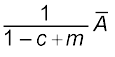 (6.9)
(6.9)
In order to examine the effects of allowing for foreign trade in the income-expenditure framework, we need to compare equation (6.10) with the equivalent expression for the equilibrium income in a closed economy model. In both equations, equilibrium income is expressed as a product of two terms, the autonomous expenditure multiplier and the level of autonomous expenditures. We consider how each of these change in the open economy context.
Since m, the marginal propensity to import, is greater than zero, we get a smaller multiplier in an open economy. It is given by
The open economy multiplier = ![]() =
=  (6.10)
EXAMPLE ![]() 6.2
6.2
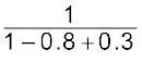
If c = 0.8 and m = 0.3, we would have the open and closed economy multiplier respectively as
 =
=  =
= ![]() = 5 (6.11)
= 5 (6.11)
and
 =
=  =
= ![]() = 2 (6.12)
= 2 (6.12)
If domestic autonomous demand increases by 100, in a closed economy output increases by 500 whereas it increases by only 200 in an open economy.
The fall in the value of the autonomous expenditure multiplier with the opening up of the economy can be explained with reference to our previous discussion of the multiplier process (Chapter 4). A change in autonomous expenditures, for instance a change in government spending, will have a direct effect on income and an induced effect on consumption with a further effect on income. With an mpc greater than zero, a proportion of the induced effect on consumption will be a demand for foreign, not domestic goods. Therefore, the induced effect on demand for domestic goods, and hence on domestic income, will be smaller. The increase in imports per unit of income constitutes an additional leakage from the circular flow of domestic income at each round of the multiplier process and reduces the value of the autonomous expenditure multiplier.
The second term in equation (6.10) shows that, in addition to the elements for a closed economy, autonomous expenditure for an open economy includes the level of exports and the autonomous component of imports. Thus, the changes in their levels are additional shocks that will change equilibrium income. From equation (6.10) we can compute the multiplier effects of changes in ![]() and
and ![]() .
.
 =
=  (6.13)
 =
=  (6.14)
An increase in demand for our exports is an increase in aggregate demand for domestically produced output and will increase demand just as would an increase in government spending or an autonomous increase in investment. In contrast, an autonomous rise in import demand is seen to cause a fall in demand for domestic output and causes equilibrium income to decline.