2
Data Processing

Measures of Central Tendency
Mean
Mode
Mode is the maximum occurrence or frequency at a particular point or value. You may notice that each one of these measures is a different method of determining a single representative number suited to different types of the data sets.
Mean
Mean is the simple arithmetic average of the different values of a variable. For ungrouped and grouped data, the methods for calculating mean are necessarily different. Mean can be calculated by direct or indirect methods, for both grouped and ungrouped data.
Computing Mean from Ungrouped Data
Direct Method
While calculating mean from ungrouped data using the direct method, the values for each observation are added and the total number of occurrences are divided by the sum of all observations. The mean is calculated using the following formula:
X̅=Σx/N
Where,![]()
X = Mean
∑ = Sum of a series of measures
x = A raw score in a series of measures
∑x =The sum of all the measures
N = Number of measures
Example 2.1 : Calculate the mean rainfall for Malwa Plateau in Madhya Pradesh from the rainfall of the districts of the region given in Table 2.1:
Table 2.1 : Calculation of Mean Rainfall
The mean for the data given in Table 2.1 is computed as under:
X̅=Σx/N
6,484/7 = 926.29
It could be noted from the computation of the mean that the raw rainfall data have been added directly and the sum is divided by the number of observations i. e., districts. Therefore, it is known as direct method.
Indirect Method
For a large number of observations, the indirect method is normally used to compute the mean. It helps in reducing the values of the observations to smaller numbers by subtracting a constant value from them. For example, as shown in Table 2.1, the rainfall values lie between 800 and 1100 mm. We can reduce these values by selecting ‘assumed mean’ and subtracting the chosen number from each value. In the present case, we have taken 800 as assumed mean. Such an operation is known as coding. The mean is then worked out from these reduced numbers (Column 3 of Table 2.1).
The following formula is used in computing the mean using indirect method:
X̅=A + Σd/N
Where,
A =Subtracted constant
Σd =Sum of the coded score
N =Number of individual observations in a series
Mean for the data as shown in Table 2.1 can be computed using the indirect method in the following manner :
X̅= 800 + 884/7
X̅= 926.29
Note that the mean value comes the same when computed either of the two methods.
Computing Mean from Grouped Data
The mean is also computed for the grouped data using either direct or indirect method.
Direct Method
When scores are grouped into a frequency distribution, the individual values lose their identity. These values are represented by the midpoints of the class intervals in which they are located. While computing the mean from grouped data using direct method, the midpoint of each class interval is multiplied with its corresponding frequency ( f ); all values of fx (the X are the midpoints) are added to obtain Σƒx that is finally divided by the number of observations i. e., N. Hence, mean is calculated using the following formula :
X̅ = Σƒx/N
Where :Example 2.2 : Compute the average wage rate of factory workers using data given in Table 2.2:
Table 2.2 : Wage Rate of Factory Workers
Table 2.3 : Computation of Mean
Where N = Σƒ = 99
Table 2.3 provides the procedure for calculating the mean for grouped data. In the given frequency distribution, ninety-nine workers have been grouped into five classes of wage rates. The midpoints of these groups are listed in the third column. To find the mean, each midpoint (X) has been multiplied by the frequency ( ƒ) and their sum (Σƒx ) divided by N.
The mean may be computed as under using the given formula :
X̅ = Σƒx/N
10,160/99 =102.6
Indirect Method
The following formula can be used for the indirect method for grouped data. The principles of this formula are similar to that of the indirect method given for ungrouped data. It is expressed as under
X̅= A ± Σƒd/N
Where,
A = Midpoint of the assumed mean group
(The assumed mean group in Table 2.3 is 90 – 110 with 100 as midpoint.)
ƒ = Frequency
d = Deviation from the assumed mean group (A)
N = Sum of cases or ∑ f
i = Interval width (in this case, it is 20)
From Table 2.3 the following steps involved in computing mean using the direct method can be deduced :
1. Mean has been assumed in the group of 90 – 110. It is preferably assumed from the class as near to the middle of the series as possible. This procedure minimises the magnitude of computation. In Table 2.3, A (assumed mean) is 100, the midpoint of the class 90 – 110.2. The fifth column (u) lists the deviations of midpoint of each class from the midpoint of the assumed mean group (90 – 110).
3 .The sixth column shows the multiplied values of each f by its corresponding d to give fd. Then, positive and negative values of fd are added separately and their absolute difference is found (∑ fd ). Note that the sign attached to ∑ fd is replaced in the formula following A, where ± is given.
The mean using indirect method is computed as under :
X̅= A ± Σƒd/N
=100 +260/99
=100+ 2.6
=102.6
Note : The Indirect mean method will work for both equal and unequal class intervals.
Median
Median is a positional average. It may be defined “as the point in a distribution with an equal number of cases on each side of it”. The Median is expressed using symbol M.
Computing Median for Ungrouped Data
When the scores are ungrouped, these are arranged in ascending or descending order. Median can be found by locating the central observation or value in the arranged series. The central value may be located from either end of the series arranged in ascending or descending order. The following equation is used to compute the median :
Value of (N+1/2) th item
Example 2.3: Calculate median height of mountain peaks in parts of the Himalayas using the following:
8,126 m, 8,611m, 7,817 m, 8,172 m, 8,076 m, 8,848 m, 8,598 m.
Computation : Median (M) may be calculated in the following steps :
1. Arrange the given data in ascending or descending order.2. Apply the formula for locating the central value in the series. Thus :
Value of (N+1/2) th item
(7+1/2)th item
4th item in the arranged series will be the Median.
Arrangement of data in ascending order –
Hence,
M = 8,172 m
Computing Median for Grouped Data
When the scores are grouped, we have to find the value of the point where an individual or observation is centrally located in the group. It can be computed using the following formula :
M = l + i/ƒ (N/2 - C)
Where,
M = Median for grouped data
l = Lower limit of the median class
i = Interval
ƒ = Frequency of the median class
N = Total number of frequencies or number of observations
c = Cumulative frequency of the pre-median class.
Example 2.4 : Calculate the median for the following distribution :
Table 2.4 : Computation of Median
The median is computed in the steps given below :
(i) The frequency table is set up as in Table 2.4.
(ii) Cumulative frequencies (F) are obtained by adding each normal frequency of the successive interval groups, as given in column 3 of Table 2.4.
(iii) Median number is obtained by N/2 i.e. 50/2 = 25 in this case, as shown in column 4 of Table 2.4.
(iv) Count into the cumulative frequency distribution (F) from the top towards bottom until the value next greater than N/2 is reached. In this example, N/2 is 25, which falls in the Class interval of 40-44 with cumulative frequency of 37, thus the cumulative frequency of the premedian class is 21 and actual frequency of the median class is 16.
(v) The median is then computed by substituting all the values determined
in the step 4 in the following equation :
M = l + i/ƒ(m-c)
= 80 + 10/16(25-21)
= 80 + 5/8 x 4
= 80 + 5/2
= 80 + 2.5
M = 82.5
Mode
The value that occurs most frequently in a distribution is referred to as mode. It is symbolised as Z or M0 . Mode is a measure that is less widely used compared to mean and median. There can be more than one type mode in a given data set.
Computing Mode for Ungrouped Data
While computing mode from the given data sets all measures are first arranged in ascending or descending order. It helps in identifying the most frequently occurring measure easily.
Example 2.5 : Calculate mode for the following test scores in geography for ten students :
61, 10, 88, 37, 61, 72, 55, 61, 46, 22
Computation : To find the mode the measures are arranged in ascending order as given below:
10, 22, 37, 46, 55, 61, 61, 61, 72, 88.
The measure 61 occurring three times in the series is the mode in the given dataset. As no other number is in the similar way in the dataset, it possesses the property of being unimodal.
Example 2.6 : Calculate the mode using a different sample of ten other students, who scored:
82, 11, 57, 82, 08, 11, 82, 95, 41, 11.
Computation : Arrange the given measures in an ascending order as shown below :
08, 11, 11, 11, 41, 57, 82, 82, 82, 95
It can easily be observed that measures of 11 and 82 both are occurring three times in the distribution. The dataset, therefore, is bimodal in appearance. If three values have equal and highest frequency, the series is trimodal. Similarly, a recurrence of many measures in a series makes it multimodal. However, when there is no measure being repeated in a series it is designated as without mode.
Comparison of Mean, Median and Mode
The three measures of the central tendency could easily be compared with the help of normal distribution curve. The normal curve refers to a frequency distribution in which the graph of scores often called a bell-shaped curve. Many human traits such as intelligence, personality scores and student achievements have normal distributions. The bell-shaped curve looks the way it does, as it is symmetrical. In other words, most of the observations lie on and around the middle value. As one approaches the extreme values, the number of observations reduces in a symmetrical manner. A normal curve can have high or low data variability. An example of a normal distribution curve is given in Fig. 2.3.
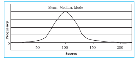
Fig. 2.3 : Normal Distribution Curve
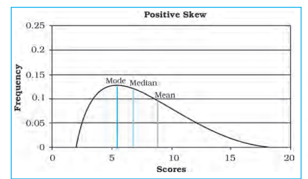
Fig. 2.4 : Positive Skew
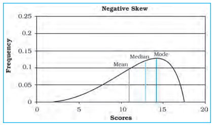
Fig. 2.5 : Negative Skew
Measures of Dispersion
The measures of Central tendency alone do not adequately describe a distribution as they simply locate the centre of a distribution and do not tell us anything about how the scores or measurements are scattered in relation to the centre. Let us use the data given in Table 2.5 and 2.6 to understand the limitations of the measures of central tendency.
Table 2.5 : Scores of Individuals
Table 2.6 : Scores of Individuals
X = 50 for both the distributions
It can be observed that the mean derived from the two data sets (Table 2.5 and 2.6) is same i. e. 50. The highest and the lowest score shown in Table 2.5 is 55 and 45 respectively. The distribution in Table 2.6 has a high score of 98 and a low score of zero. The range of the first distribution is 10, whereas, it is 98 in the second distribution. Although, the mean for both the groups is the same, the first group is obviously stable or homogeneous as compared to the distribution of score of the second group, which is highly unstable or heterogeneous. This raises a question whether the mean is a sufficient indicator of the total character of distributions. The examples provide profound evidence that it is not so. Thus, to get a better picture of a distribution, we need to use a measure of central tendency and of dispersion or variability.
The term dispersion refers to the scattering of scores about the measure of central tendency. It is used to measure the extent to which individual items or numerical data tend to vary or spread about an average value. Thus, the dispersion is the degree of spread or scatter or variation of measures about a central value.
The dispersion serves the following two basic purposes :
1. It gives us the nature of composition of a series or distribution, and2. It permits comparison of the given distributions in terms of stability or homogeneity.
Methods of Measuring Dispersion
The following methods are used as measures of dispersion :
1. Range2. Quartile Deviation
3. Mean Deviation
4. Standard Deviation and Coefficient of Variation (CV)
5. Lorenz Curve
Each of these methods has definite advantages as well as limitations. Hence, there is a need to use either of the methods with great precautions. The Standard Deviation (s) as an absolute measure of dispersion and Coefficient of Variation (CV) as a relative measure of dispersion, besides the Range are most commonly used measures of dispersion. We will discuss how each one of these measures is computed.
Range
Range (R) is the difference between maximum and minimum values in a series of distribution. This way it simply represents the distance from the smallest to the largest score in a series. It can also be defined as the highest score minus the lowest score.
Range for Ungrouped Data
Example 2.7 : Calculate the range for the following distribution of daily wages:
Rs. 40, 42, 45, 48, 50, 52, 55, 58, 60, 100.
Computation of Range
The R can be calculated with the help of the following formula :
R= L- S
Where
‘R’ is Range,
‘L’ and ‘S’ is the largest and smallest values respectively in a series.
Hence,
R = L – S
= 100 – 40= 60
If we eliminate the 10th case, R becomes 20 (60 – 40). The elimination of one score has reduced the R to just one-third. It is obvious that the difficulty with R as a measure of variability is that its value is wholly dependent upon the two extreme scores. Thus, as a measure of dispersion R functions much the same way as mode does as a measure of central tendency. Both the measures are highly unstable.
Standard Deviation
Standard deviation (SD) is the most widely used measure of dispersion. It is defined as the square root of the average of squares of deviations. It is always calculated around the mean. The standard deviation is the most stable measure of variability and is used in so many other statistical operations. The Greek character σ denotes it.
To obtain SD, deviation of each score from the mean (x) is first squared (x 2 ). It is important to note that this step makes all negative signs of deviations positive. It saves SD from the major criticism of mean deviation which uses modulus x. Then, all of the squared deviations are summed - x 2 (care should be taken that these are not summed first and then squared). This sum of the squared deviations ( x 2 ) is divided by the number of cases and then the square root is taken. Therefore, Standard Deviation is defined as the root mean square deviation. For a given data set, it is computed using the following formula :
During these steps, we come across a term before taking its square root. It is assigned a special name, the variance. The variance is widely used in advanced statistical operations. Its square root is standard deviation. That way, the opposite is also true i.e. square of SD is variance.
Standard Deviation for Ungrouped Data
Example 2.8 : Calculate the standard deviation for the following scores : Table 2.7 : Computation of
Standard Deviation 01, 03, 05, 07, 09
𝛔σ = √ ( Σx2 / N)
= √40/5
= √8 = 2.828
Let us summarise the steps used in the above computation :
1. All the scores have been placed in the column marked X.2. Summing the raw scores and dividing by N have found mean.
3. Deviation of each raw score (x) has been obtained by subtracting the mean from them. A check on our work is that the sum of the x should be zero. We find that this is true for our exercise.
4. Each value of x has been squared and summed.
5. Sum of the x 2 s has been divided by N. Recall that the resultant is the variance.
6. Its square root has been found to obtain Standard Deviation.
Computation of Standard Deviation for Grouped Data
Example : Calculate the standard deviation for the following distribution:
The method of obtaining SD for grouped data has been explained in the table below. The initial steps upto column 4, are the same as those we followed in the computation of the mean for grouped data. We begin with assuming our mean to exist in the interval group of 150-160, hence a deviation value of zero has been assigned to the group. Likewise other deviations are determined. Values in column 4 (fx´) are obtained by the multiplication of the values in the two previous columns. Values in column 5 (fx´2) are obtained by multiplying the values given in column 3 and 4. Then various columns have been summed.
The following formula is used to calculate the Standard Deviation :
SD = t2| Σƒx`2 - Σƒx`/ N
Coefficient of Variation (CV)
When the observations for different places or periods are expressed in different units of measurement and are to be compared, the coefficient of variation (CV) proves very useful. CV expresses the standard deviation as a percentage of the mean. It is determined using the following formula :
Standard Deviation
CV = Standard/Mean x100
The CV for the dataset given in Table 2.7 will, hence, be as under :
CV = σ/X̅ x 100
CV = 2.83 /5 x 100
CV= 56%
Coefficient of Variation for grouped data can also be calculated using the same formula.
Rank Correlation
The statistical methods discussed so far were concerned with the analysis of a single variable. We will now discuss the methods of exploring relationship between two variables and the way this relationship is expressed numerically. When dealing with two or more sets of data, curiosity arises for knowing whether or not changes in one variable produce changes in some other variable.Often our interest lies in knowing the nature of relationship or interdependence between two or more sets of data. It has been found that the correlation serves useful purpose. It is basically a measure of relationship between two or more sets of data. Since, we study the way they vary, we call these events variables. Thus, the term correlation refers to the nature and strength of correspondence or relationship between two variables. The terms nature and strength in the definition refer to the direction and degree of the variables with which they co-vary.
Direction of Correlation
It is our common experience that an input is made to get some output. There could be three possibilities.
1. With the increase in input the output also increases.2. With the increase in the input the output decreases.
3. Change in the input does not lead to change in the output.
In the first case, the direction of the relationship between the input and output is in the same direction. It is called that both are positively correlated.
In the second case the direction of change between the input and output is in the opposite direction and it is called that they are negatively correlated.
In the third case, change in the input has no relationship with the output, hence, it is said that these do not have a statistically significant relationship.
Let us now consider Fig. 2.7 which looks just opposite of Fig. 2.6. The plotted values run from the upper left to the lower right of the graph. Notice that for every increase of one unit on the X-axis, there is a corresponding decrease of two units on the Y-axis. It is an example of a negative correlation. It means that the two variables have a tendency to move opposite to each other, i.e. if one variable increases, the other decreases and vice versa. We can find such relationships existing between various geographical pairs of variables. Correlations betweenb height above sea level and air pressure, temperature and air pressure are a few examples. It implies that the obtained figure of correlation must precede with the arithmetical sign (plus or minus), more importantly in the negative correlation.
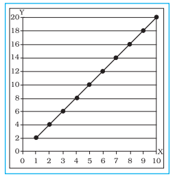
Fig. 2.6 : Perfect Positive
Correlation
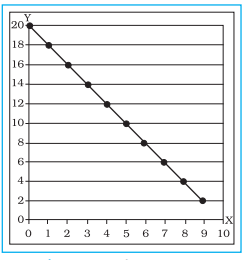
Fig. 2.7 : Perfect Negative
Correlation
Degree of Correlation
When reference has been made about the direction of correlation, negative or
positive, a natural curiosity arises to know the degree of correspondence or
association of the two variables. The maximum degree of correspondence or
relationship goes upto 1 (one) in mathematical terms. On adding an element of
the direction of correlation, it spreads to the maximum extent of –1 to +1
through zero. It can never be more than one. The spread can also be translated
into linear shape, as shown in the Fig. 2.8. Correlation of 1 is known as perfect
correlation (whether positive and negative). Between the two points of divergent,
perfect correlations lies 0 (zero) correlation, a point of no correlation or absence
of any correlation between the variables.
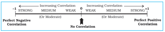
Fig. 2.8 : Spread of Direction and Degree of Correlation
Fig. 2.7 is just opposite of this. All the points again fall along a straight line which now runs from the upper left-hand part of the scatter gram to its lower right. It is an example of a perfect negative correlation (with a value of – 1.00). No Correlation (or Zero Correlation) is one when any of the variables in the pair does not respond to the changes in the other, the correlation will come to zero. This is the state of no correlation or zero correlation. This is shown in Fig. 2.9. Scatter plot A shows no correlation when Y does not respond to changes in X. Similarly, zero correlation occurs in Seatter plot B when X does not respond to changes in Y.
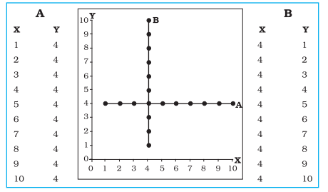
Fig. 2.9 : Scatter plot showing No Correlation
Other Correlations
Between the perfect correlations (±1) and zero correlation lies generalised conditions popularly referred to as weak, moderate and strong correlations. These conditions are clearly exhibited in Figs. 2.10, 2.11 and 2.12 respectively. Notice the spreading or the scattering of the plotted points and the assignment of the terms weak, medium and strong to them (generalised terms having no specific limits). Larger is the scattering, weaker is the correlation. Smaller is the scattering, stronger is the correlation, and when the plotted points fall on a straight line, the correlation is perfect (Fig. 2.6 and 2.7).
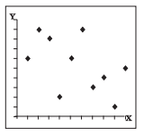
Fig. 2.10 : Weak
Negative Correlation
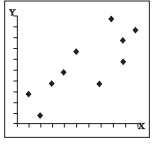
Fig. 2.11 : Moderate
Positive Correlation
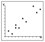
Fig. 2.12 : Strong
Positive Correlation
Methods of Calculating Correlation
There are various methods by which correlation can be calculated. However, under the constraints of time and space, we will discuss the Spearman’s Rank Correlation method only.
Spearman’s Rank Correlation
Spearman devised a method of computing correlation with the help of ranks. The method is popularly known as Spearman’s Rank Correlation symbolised asr ρ (the Greek letter rho). Spearman’s Rank Correlation method is widely used. The computation of the correlation is undertaken in the steps given below:
1. Copy the data related to X-Y variables given in the exercise and put them in the first and second columns of the table.2. Both the variables are to be ranked separately. The ranks of X-variable are to be recorded in column 3 headed by XR (ranks of X). Similarly, the ranks of Y-variable (YR) are to be recorded in the fourth column. The highest value in the data is to be awarded rank one, second highest rank two and so on. Suppose the data for X-variable are 4, 8, 2, 10, 1,9, 7, 3, 0 and 5, the XR will be 6, 3, 8, 1, 9, 2, 4, 7, 10 and 5 respectively. Notice that the last rank (10 in this case) equals the number of observations. Assignment of YR is also done in the same way.
3. Now since both XR and YR have been obtained, find the difference between the two sets of ranks (disregarding the sign plus or minus) and record it in the fifth column. The sign of the difference is of no importance, since, these differences are squared in the next operation.
4. Each of these differences is squared and sum of this column of squares is obtained. These values are placed in the sixth column.
5. Then the computation of the rank correlation is done by the application of the following equation:
ρ = 1- 6 Σ D2/ N(N2-1)
Where,
ρ = rank correlation
∑D 2 = sum of the squares of the differences between two sets of ranks N = the number of pairs of X-Y
Example 2.9: Calculate Spearman’s Rank Correlation with the help of the following data :
Table 2.8 : Computation of Spearman’s Rank Correlation
Calculation:
Where, ρ is Rank Correlation; D is difference between the rank of X and Y; and
N is number of items of x – y
ρ = 1- 6 Σ D2/ N(N2-1)
= 1 - 6 x 8/10(10 2 - 1)
=1 -48/10(100-1)
=1 - 48/10(99)
=1 - 48/(990)
= 1- 0.05
= 0.95
In rho, we obtain a correlation, which makes a good substitute for other types of correlations, when the number of cases is small. It is almost useless when N is large, because by the time all the data are ranked, other type of correlation could have been calculated.
Excercises
1. Choose the correct answer from the four alternatives given below:(ii) The measure of central tendency always coinciding with the hump of any distribution is:
(iii) A scatter plot represents negative correlation if the plotted values run from:
2. Answer the following questions in about 30 words:
2. What are the advantages of using mode ?
3. What is dispersion ?
4. Define correlation.
5. What is perfect correlation ?
6. What is the maximum extent of correlation?
2. Comment on the applicability of mean, median and mode (hint: from their merits and demerits).
3. Explain the process of computing Standard Deviation with the help of an imaginary example.
4. Which measure of dispersion is the most unstable statistic and why?
5. Write a detailed note on the degree of correlation.
6. What are various steps for the calculation of rank order correlation?
Activity
1. Take an imaginary example applicable to geographical analysis and explain direct and indirect methods of calculating mean from ungrouped data.2. Draw scatter plots showing different types of perfect correlations.