Table of Contents

6
Non-competitive Markets
We recall that perfect competition is a market structure where both consumers and firms are price takers. The behaviour of the firm in such circumstances was described in the Chapter 4. We discussed that the perfect competition market structure is approximated by a market satisfying the following conditions:
(i) there exist a very large number of firms and consumers of the commodity, such that the output sold by each firm is negligibly small compared to the total output of all the firms combined, and similarly, the amount purchased by each consumer is extremely small in comparison to the quantity purchased by all consumers together;
(ii) firms are free to start producing the commodity or to stop production; i.e., entry and exit is free
(iii) the output produced by each firm in the industry is indistinguishable from the others and the output of any other industry cannot substitute this output; and
(iv) consumers and firms have perfect knowledge of the output, inputs and their prices.
In this chapter, we shall discuss situations where one or more of these conditions are not satisfied. If assumption (ii) is dropped, and it becomes difficult for firms to enter a market, then a market may not have many firms. In the extreme case a market may have only one firm. Such a market, where there is one firm and many buyers is called a monopoly. A market that has a small number of large firms is called an oligopoly. Notice that dropping assumption (ii) leads to dropping assumption (i) as well. Similarly, dropping the assumption that goods produced by a firm are indistinguishable from those of other firms (assumption iii) implies that goods produced by firms are close substitutes, but not perfect substitutes for each other. Such markets, where assumptions (i) and (ii) may hold, but (iii) does not hold are called markets with monopolistic competition. This chapter examines the market structures of monopoly, monopolistic competition and oligopoly.
6.1 Simple Monopoly in the Commodity Market
A market structure in which there is a single seller is called monopoly. The conditions hidden in this single line definition, however, need to be explicitly stated. A monopoly market structure requires that there is a single producer of a particular commodity; no other commodity works as a substitute for this commodity; and for this situation to persist over time, sufficient restrictions are required to be in place to prevent any other firm from entering the market and to start selling the commodity.
In order to examine the difference in the equilibrium resulting from a monopoly in the commodity market as compared to other market structures, we also need to assume that all other markets remain perfectly competitive. In particular, we need (i) All the consumers are price takers; and (ii) that the markets of the inputs used in the production of this commodity are perfectly competitive both from the supply and demand side.
‘I’ ‘M’ Perfect Competition
If all the above conditions are satisfied, then we define the situation as one of monopoly in a single commodity market.
Competitive Behaviour versus Competitive Structure
A perfectly competitive market has been defined as one where an individual firm is unable to influence the price at which the product is sold in the market. Since price remains the same for any level of output of the individual firm, such a firm is able to sell any quantity that it wishes to sell at the given market price. It, therefore, does not need to compete with other firms to obtain a market for its produce.
This is clearly the opposite of the meaning of what is commonly understood by competition or competitive behaviour. We see that Coke and Pepsi compete with each other in a variety of ways to achieve a higher level of sales or a greater share of the market. Conversely, we do not find individual farmers competing among themselves to sell a larger amount of crop. This is because both Coke and Pepsi possess the power to influence the market price of soft drinks, while the individual farmer does not.
Thus, competitive behaviour and competitive market structure are, in general, inversely related; the more competitive the market structure, less competitive is the behaviour of the firms. On the other hand, the less competitive the market structure, the more competitive is the behaviour of firms towards each other. In a monopoly there is no other firm to compete with.
6.1.1 Market Demand Curve is the Average Revenue Curve
The market demand curve in Figure 6.1 shows the quantities that consumers as a whole are willing to purchase at different prices. If the market price is at p0, consumers are willing to purchase the quantity q0. On the other hand, if the market price is at the lower level p1, consumers are willing to buy a higher quantity q1. That is, price in the market affects the quantity demanded by the consumers. This is also expressed by saying that the quantity purchased by the consumers is a decreasing function of the price. For the monopoly firm, the above argument expresses itself from the reverse direction. The monopoly firm’s decision to sell a larger quantity is possible only at a lower price. Conversely, if the monopoly firm brings a smaller quantity of the commodity into the market for sale it will be able to sell at a higher price. Thus, for the monopoly firm, the price depends on the quantity of the commodity sold. The same is also expressed by stating that price is a decreasing function of the quantity sold. Thus, for the monopoly firm, the market demand curve expresses the price that consumers are willing to pay for different quantities supplied. This idea is reflected in the statement that the monopoly firm faces the market demand curve, which is downward sloping.
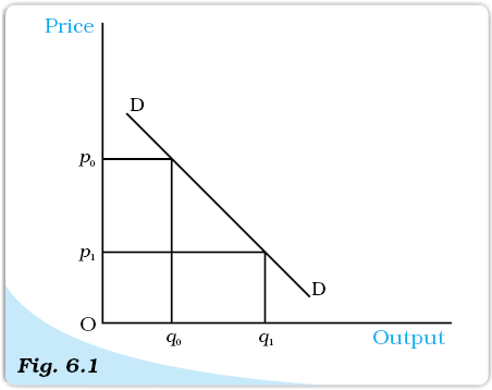
Market Demand Curve. Shows the quantities that consumers as a whole are willing to purchase at different prices.
The above idea can be viewed from another angle. Since the firm is assumed to have perfect knowledge of the market demand curve, the monopoly firm can decide the price at which it wishes to sell its commodity, and therefore, determines the quantity to be sold. For instance, examining Figure 6.1 again, since the monopoly firm is aware of the shape of the curve DD, if it wishes to sell the commodity at the price p0, it can do so by producing and selling quantity q0, since at the price p0, consumers are willing to purchase the quantity q0. On the other hand, if it wants to sell q1, it will only be able to do so at the price p1.
The contrast with the firm in a perfectly competitive market structure should be clear. In that case, the firm could bring into the market as much quantity of the commodity as it wished and could sell it at the same price. Since this does not happen for a monopoly firm, the amount received by the firm through the sale of the commodity has to be examined again.
We do this exercise through a schedule, a graph, and using a simple equation of a straight line demand curve. As an example, let the demand function be given by the equation
q = 20 – 2p,
where q is the quantity sold and p is the price in rupees.
The equation can be written in terms of p as
p = 10 – 0.5q
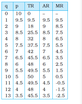
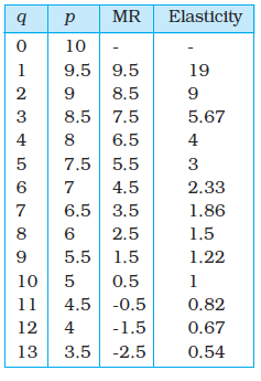
Substituting different values of q from 0 to 13 gives us the prices from 10 to 3.5. These are shown in the q and p columns of Table 6.1.
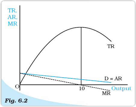
These numbers are depicted in a graph in Figure 6.2 with prices on the vertical axis and quantities on the horizontal axis. The prices that are available for different quantities of the commodity are shown by the solid straight line D.
The total revenue (TR) received by the firm from the sale of the commodity equals the product of the price and the quantity sold. In the case of the monopoly firm, the total revenue is not a straight line. Its shape depends on the shape of the demand curve. Mathematically, TR is represented as a function of the quantity sold. Hence, in our example
TR = p × q
= (10 – 0.5q) × q
= 10q – 0.5q2
This is not the equation of a straight line. It is a quadratic equation in which the squared term has a negative cofficient. Such an equation represents an inverted vertical parabola.
Total, Average and Marginal Revenue Curves: The total revenue, average revenue and the marginal revenue curves are depicted here.
In Table 6.1, the TR column represents the product of the p and q columns. It can be noticed that as the quantity increases, TR increases to Rs 50 when output becomes 10 units, and after this level of output, total revenue starts declining. The same is visible in Figure 6.2.
The revenue received by the firm per unit of commodity sold is called the Average Revenue (AR). Mathematically, AR = TR/q. In Table 6.1, the AR column provides values obtained by dividing TR values by q values. It can be seen that the AR values turn out to be the same as the values in the p column. This is only to be expected
As seen earlier, the p values represent the market demand curve as shown in Figure 6.2. The AR curve will therefore lie exactly on the market demand curve. This is expressed by the statement that the market demand curve is the average revenue curve for the monopoly firm.
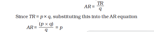
Relation between Average Revenue and Total Revenue Curves. The average revenue at any level of output is given by the slope of the line joining the origin and the point on the total revenue curve corresponding to the output level under consideration.
Graphically, the value of AR can be found from the TR curve for any level of quantity sold through a simple construction given in Figure 6.3. When quantity is 6 units, draw a vertical line passing through the value 6 on the horizontal axis. This line will cut the TR curve at the point marked ‘a’ at a height equal to 42. Draw a straight line joining the origin O and point ‘a’. The slope of this ray from the origin to a point on the TR provides the value of AR. The slope of this ray is equal to 7. Therefore, AR has the value 7. The same can be verified from Table 6.1.
6.1.2 Total, Average and Marginal Revenues
A more careful glance at Table 6.1 reveals that TR does not increase by the same amount for every unit increase in quantity. Sale of the first unit leads to a change in TR from Rs 0 when quantity is of 0 unit to Rs 9.50 when quantity is 1 unit, i.e., a rise of Rs 9.50. As the quantity increases further, the rise in TR is smaller. For example, for the 5th unit of the commodity, the rise in TR is
Rs 5.50 (Rs 37.50 for 5 units minus Rs 32 for 4 units). As mentioned earlier, after 10 units of output, TR starts declining. This implies that bringing more than 10 units for sale leads to a level of TR less than Rs 50. Thus, the rise in TR due to the 12th unit is: 48 – 49.50 = –1.5, ie a fall of Rs 1.50.
This change in TR due to the sale of an additional unit is termed Marginal Revenue (MR). In Table 6.1, this is depicted in the last column. Observe that the MR at any quantity is the difference between the TR at that quantity and the TR at the previous quantity. For example, when q = 3, MR = (25.5 – 18) = 7.5
In the last paragraph, it was shown that TR increases more slowly as quantity sold increases and falls after quantity reaches 10 units. The same can be viewed through the MR values which fall as q increases. After the quantity reaches 10 units, MR has negative values. In Figure 6.2, MR is depicted by the dotted line.
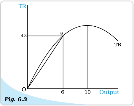
Relation between Marginal Revenue and Total Revenue Curves. The marginal revenue at any level of output is given by the slope of the total revenue curve at that level of output.
Graphically, the values of the MR curve are given by the slope of the TR curve. The slope of any smooth curve is defined as the slope of the tangent to the curve at that point. This is depicted in Figure 6.4. At point ‘a’ on the TR curve, the value of MR is given by the slope of the line L1, and at point ‘b’ by the line L2. It can be seen that both lines have positive slope, but the line L2 is flatter than line L1, ie its slope is lesser. When 10 units of the commodity are sold, the tangent to the TR is horizontal, ie its slope is zero.1 The value of the MR for the same quantity is zero. At point ‘d’ on the TR curve, where the tangent is negatively sloped, the MR takes a negative value.
We can now conclude that when total revenue is rising, marginal revenue is positive, and when total revenue shows a fall, marginal revenue is negative.
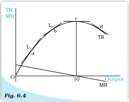
Another relation can be seen between the AR and the MR curves. Figure 6.2 shows that the MR curve lies below the AR curve. The same can be seen in Table 6.1 where the values of MR at any level of output are lower than the corresponding values of AR. We can conclude that if the AR curve (ie the demand curve) is falling steeply, the MR curve is far below the AR curve. On the other hand, if the AR curve is less steep, the vertical distance between the AR and MR curves is smaller. Figure 6.5(a) shows a flatter AR curve while Figure 6.5(b) shows a steeper AR curve. For the same units of the commodity, the difference between AR and MR in panel (a) is smaller than the difference in panel (b).
Relation between Average Revenue and Marginal Revenue curves. If the AR curve is steeper, then the MR curve is far below the AR curve.
6.1.3 Marginal Revenue and Price Elasticity of Demand
The MR values also have a relation with the price elasticity of demand. The detailed relation is not derived here. It is sufficient to notice only one aspect– price
elasticity of demand is more than 1 when the MR has a positive value, and becomes less than the unity when MR has a negative value. This can be seen in Table 6.2, which uses the same data presented in Table 6.1. As the quantity of the commodity increases, MR value becomes smaller and the value of the price elasticity of demand also becomes smaller. Recall that the demand curve is called elastic at a point where price elasticity is greater than unity, inelastic at a point where the price elasticity is less than unity and unitary elastic when price elasticity is equal to 1. Table 6.2 shows that when quantity is less than 10 units, MR is positive and the demand curve is elastic and when quantity is of more than 10 units, the demand curve is inelastic. At the quantity level of 10 units, the demand curve is unitary elastic.
Table 6.2: MR and Price Elasticity
6.1.4 Short Run Equilibrium of the Monopoly Firm
As in the case of perfect competition, we continue to regard the monopoly firm as one which maximises profit. In this section, we analyse this profit maximising behaviour to determine the quantity produced by a monopoly firm and price at which it is sold. We shall assume that a firm does not maintain stocks of the quantity produced and that the entire quantity produced is put up for sale.
The Simple Case of Zero Cost
Suppose there exists a village situated sufficiently far away from other villages. In this village, there is exactly one well from which water is available. All residents are completely dependent for their water requirements on this well. The well is owned by one person who is able to prevent others from drawing water from it except through purchase of water. The person who purchases the water has to draw the water out of the well. The well owner is thus a monopolist firm which bears zero cost in producing the good. We shall analyse this simple case of a monopolist bearing zero costs to determine the amount of water sold and the price at which it is sold.
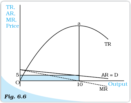
Short Run Equilibrium of the Monopolist with Zero Costs. The monopolist’s profit is maximised at that level of output for which the total revenue is the maximum.
Figure 6.6 depicts the same TR, AR and MR curves, as in Figure 6.2. The profit received by the firm equals the revenue received by the firm minus the cost incurred, that is, Profit = TR – TC. Since in this case TC is zero, profit is maximum when TR is maximum. This, as we have seen earlier, occurs when output is of 10 units. This is also the level when MR equals zero. The amount of profit is given by the length of the vertical line segment from ‘a’ to the horizontal axis.
The price at which this output will be sold is the price that the consumers as a whole are willing to pay. This is given by the market demand curve D. At output level of 10 units, the price is Rs 5. Since the market demand curve is the AR curve for the monopolist firm, Rs 5 is the average revenue received by the firm. The total revenue is given by the product of AR and the quantity sold, ie Rs 5 × 10 units = Rs 50. This is depicted by the area of the shaded rectangle.
Comparison with Perfect Competition
We compare the above outcome with what it would be under perfectly competitive market structure. Let us assume that there is an infinite number of such wells. Suppose a well-owner decides to charge Rs.5/bucket of water. Who will buy from him? Remember that there are many, many well-owners. Any other well-owner can attract all the buyers willing to buy for Rs. 5/bucket, by offering to sell to them at a lower price, say, Rs. 4/bucket.. Some other well-owner can offer to sell at a still lower price, and the story will repeat itself. In fact, competition among well-owners will drive the price down to zero. At this price 20 buckets of water will be sold.
Through this comparison, we can see that a perfectly competitive equilibrium results in a larger quantity being sold at a lower price. We can now proceed to the general case involving positive costs of production.
Introducing Positive Costs
Analysing using Total curves
In Chapter 3, we have discussed the concept of cost and the shape of the total cost curve having been depicted as shown by TC in Figure 6.7. The TR curve is also drawn in the same diagram. The profit received by the firm equals the total revenue minus the total cost. In the figure, we can see that if quantity q1 is produced, the total revenue is TR1 and total cost is TC1. The difference, TR1 – TC1, is the profit received. The same is depicted by the length of the line segment AB, i.e., the vertical distance between the TR and TC curves at q1 level of output. It should be clear that this vertical distance changes for diferent levels of output. When output level is less than q2, the TC curve lies above the TR curve, i.e., TC is greater than TR, and therefore profit is negative and the firm makes losses.
The same situation exists for output levels greater than q3. Hence, the firm can make positive profits only at output levels between q2 and q3, where TR curve lies above the TC curve. The monopoly firm will choose that level of output which maximises its profit. This would be the level of output for which the vertical distance between the TR and TC is maximum and TR is above the TC, i.e., TR – TC is maximum. This occurs at the level of output q0.
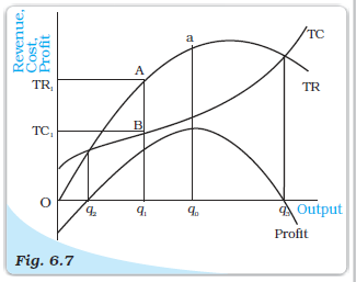
Equilibrium of the Monopolist in terms of the Total Curves. The monopolist’s profit is maximised at the level of output for which the vertical distance between the TR and TC is a maximum and TR is above the TC.
If the difference TR – TC is calculated and drawn as a graph, it will look as in the curve marked ‘Profit’ in Figure 6.7. It should be noticed that the Profit curve has its maximum value at the level of output q0. The price at which this output is sold is the price consumers are willing to pay for this q0 quantity of the commodity. So the monopoly firm will charge the price corresponding to the quantity level q0 on the demand curve.
Using Average and Marginal curves
The analysis shown above can also be conducted using Average and Marginal Revenue and Average and Marginal Cost. Though a bit more complex, this method is able to exhibit the process in greater light.
In Figure 6.8, the Average Cost (AC), Average Variable Cost (AVC) and Marginal Cost (MC) curves are drawn along with the Demand (Average Revenue) Curve and Marginal Revenue crve.
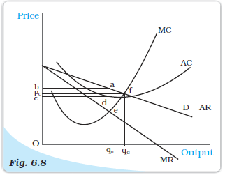
Equilibrium of the Monopolist in terms of the Average and the Marginal Curve. The monopolist’s profit is maximised at that level of output for which the MR = MC and the MC is rising.
It may be seen that at quantity level below q0, the level of MR is higher than the level of MC. This means that the increase in total revenue from selling an extra unit of the commodity is greater than the increase in total cost for producing the additional unit. This implies that an additional unit of output would create additional profits since Change in profit = Change in TR – Change in TC. Therefore, if the firm is producing a level of output less than q0, it would desire to increase its output since that would add to its profits. As long as the MR curve lies above the MC curve, the reasoning provided above would apply and thus the firm would increase its output. This process comes to a halt when the firm reaches an output level of q0 since at this level MR equals MC and increasing output provides no increase in profits.
On the other hand, if the firm was producing a level of output which is greater than q0, MC is greater than MR. This means that the lowering of total cost by reducing one unit of output is greater than the loss in total revenue due to this reduction. It is therefore advisable for the firm to reduce output. This argument would hold good as long as the MC curve lies above the MR curve, and the firm would keep reducing its output. Once output level reaches q0, the values of MC and MR become equal and the firm stops reducing its output.
At qo the firm will make maximum profits. It has no incentive to change from qo. This level is called the equilibrium level of output. Since this equilibrium level of output corresponds to the point where the MR equals MC, this equality is called the equilibrium condition for the output produced by a monopoly firm.
At this equilibrium level of output q0, the average cost is given by the point ‘d’ where the vertical line from q0 cuts the AC curve. The average cost is thus given by the height dq0. Since total cost equals the product of AC and the quantity produced being q0, the same is given by the area of the rectangle Oq0dc.
As shown earlier, once the quantity of output produced is determined, the price at which it is sold is given by the amount that the consumers are willing to pay, as expressed through the market demand curve. Thus, the price is given by the point ‘a’ where the vertical line through q0 meets the market demand curve D. This provides price given by the height aq0. Since the price received by the firm is the revenue per unit of output, it is the Average Revenue for the firm. The total revenue being the product of AR and the level of output q0, can be shown as the area of the rectangle Oq0ab.
It can be seen from the diagram that the area of the rectangle Oq0ab is larger than the area of the rectangle Oq0dc, i.e., TR is greater than TC. The difference is the area of the rectangle cdab. Thus, Profit = TR – TC which can be represented by this area cdab.
Comparison with Perfect Competition again
We compare the monopoly firm’s equilibrium quantity and price with that of the perfectly competitive firm. Recall that the perfectly competitive firm was a price taker. Given the market price, the firm in a perfectly competitive market structure believed that it could not alter the price by producing more of the output or less of it.
Suppose that the firm, whose equilibrium we were considering above, believed that it was a perfectly competitive firm. Then, given its level of output at q0, price of the commodity at aq0 = Ob, it would expect the price to remain fixed at Ob, and therefore, every additional unit of output could be sold at that price. Since the cost of producing an additional unit, given by the MC, stands at eq0 which is less than aq0, the firm would expect a gain in profit by increasing the output. This would continue as long as the price remained higher than the MC. At the point ‘f’ in Figure 6.8, where the MC curve cuts the demand curve, price received by the firm becomes equal to the MC. Hence, it would no longer be considered beneficial by this perfectly competitive firm to increase output. It is for this reason that Price = Marginal Cost that is considered the equilibrium condition for the perfectly competitive firm.
The diagram shows that at this level of output, the quantity produced qc is greater than q0. Also, the price paid by the consumers is lower at pc. From this we conclude that the perfectly competitive market provides a production and sale of a larger quantity of the commodity compared to a monopoly firm. Further the price of the commodity under perfect competition is lower compared to monopoly. The profit earned by the perfectly competitive firm is also smaller.
In the Long Run
We saw in Chapter 5 that with free entry and exit, perfectly competitive firms obtain zero profits. That was due to the fact that if profits earned by firms were positive, more firms would enter the market and the increase in output would bring the price down, thereby decreasing the earnings of the existing firms. Similarly, if firms were facing losses, some firms would close down and the reduction in output would raise prices and increase the earnings of the remaining firms. The same is not the case with monopoly firms. Since other firms are prevented from entering the market, the profits earned by monopoly firms do not go away in the long run.
Some Critical Views
We have seen how a monopoly will typically charge higher prices than a competitive firm. In this sense, monopolies are often considered exploitative.
However, varying views have been expressed by economists concerning the question of monopoly. First, it can be argued that monopoly of the kind described above cannot exist in the real world. This is because all commodities are, in a sense, substitutes for each other. This in turn is because of the fact that all the firms producing commodities, in the final analysis, compete to obtain the income in the hands of consumers.
Another argument is that even a firm in a pure monopoly situation is never without competition. This is because the economy is never stationary. New commodities using new technologies are always coming up, which are close substitutes for the commodity produced by the monopoly firm. Hence, the monopoly firm always has competition in the long run. Even in the short run, the threat of competition is always present and the monopoly firm is unable to behave in the manner we have described above.
Still another view argues that the existence of monopolies may be beneficial to society. Since monopoly firms earn large profits, they possess sufficient funds to take up research and development work, something which the small perfectly competitive firm is unable to do. By doing such research, monopoly firms are able to produce better quality goods, or goods at lower cost, or both. While it is true that monopolies make supernormal profits, they may benefit consumers by lowering costs.
6.2 Other Non-perfectly Competitive Markets
6.2.1 Monopolistic Competition
We now consider a market structure where the number of firms is large, there is free entry and exit of firms, but the goods produced by them are not homogeneous. Such a market structure is called monopolistic competition.
This kind of a structure is more commonly visible. There is a very large number of biscuit producing firms, for example. But many of the biscuits being produced are associated with some brand name and are distinguishable from one another by these brand names and packaging and are slightly different in taste. The consumer develops a taste for a particular brand of biscuit over time, or becomes loyal to a particular brand for some reason, and is, therefore, not immediately willing to substitute it for another biscuit. However, if the price difference becomes large, the consumer would be willing to choose a biscuit of another brand. A consumers’ preference for a brand will often vary in depth, so the change in price required for the consumer to change her brand may vary. Therefore, if price of a particular brand is lowered, some consumers will shift to consuming that brand. Lowering of the price further will lead to more consumers shifting to the brand with the lower price.
Hence, the demand curve faced by the firm is not horizontal (perfectly elastic) as is the case with perfect competition. The demand curve faced by the firm is also not the market demand curve, as in the case with monopoly. In the case of monopolistic competition, the firm expects increases in demand if it lowers the price. Recall that the demand curve of a firm is also its AR curve. This firm, therefore has downward sloping AR curve. The marginal revenue is less than the average revenue, and also downward sloping. The firm increases its output whenever the marginal revenue is greater than the marginal cost. What does this firm’s equilibrium look like? The monopolistic competitive firm is also a profit maximizer. So it will increase production as long as the addition to its total revenue is greater than the addition to its total costs. In other words, this firm (like the perfectly competitive firm as well as the monopoly) will choose to produce the quantity that equates its marginal revenue to its marginal cost. How does this quantity compare with that of the perfectly competitive firm? Recall that the MR for a perfectly competitive firm is equal to its AR. So the perfectly competitive firm, in an identical situation, would equate its AR to MC. So a firm under monopolistic competition will produce less than the perfectly competitive firm. Given lower output, the price of the commodity becomes higher than the price under perfect competition.
The situation described above is one that exists in the short run. But the market structure of monopolistic competition allows for new firms to enter the market. If the firms in the industry are receiving supernormal profit in the short run, this will attract new firms. As new firms enter, some customers shift from existing firms to these new firms. So existing firms find that their demand curve has shifted leftward, and the price that they receive falls. This causes profits to fall. The process continues till super-normal profits are wiped out, and firms are making only normal profits. Conversely, if firms in the industry are facing losses in the short run, some firms would stop producing (exit from the market). The demand curve for existing firms would shift rightward. This would lead to a higher price, and profit. Entry or exit would halt once supernormal profits become zero and this would serve as the long run equilibrium.
6.2.2 How do Firms behave in Oligopoly?
If the market of a particular commodity consists of more than one seller but the number of sellers is few, the market structure is termed oligopoly. The special case of oligopoly where there are exactly two sellers is termed duopoly. In analysing this market structure, we assume that the product sold by the two firms is homogeneous and there is no substitute for the product, produced by any other firm.
Given that there are a few firms, each firm is relatively large when compared to the size of the market. As a result each firm is in a position to affect the total supply in the market, and thus influence the market price. For example, if the two firms in a duopoly are equal in size, and one of them decides to double its output, the total supply in the market will increase substantially, causing the price to fall. This fall in price affects the profits of all firms in the industry. Other firms will respond to such a move in order to protect their own profits, by taking fresh decisions regarding how much to produce. Therefore the level of output in the industry, the level of prices, as well as the profits, are outcomes of how firms are interacting with each other.
At one extreme, firms could decide to ‘collude’ with each other to maximize collective profits. In this case, the firms form a ‘cartel’ that acts as a monopoly. The quantity supplied collectively by the industry and the price charged are the same as a single monopolist would have done.
At the other extreme, firms could decide to compete with each other. For example, a firm may lower its price a little below the other firms, in order to attract away their customers. Obviously, the other firms would retaliate by doing the same. So the market price keeps falling as long as firms keep undercutting each others’ prices. If the process continues to its logical conclusion, the price will have fallen till the marginal cost. (No firm will supply at a lower price than the marginal cost). Recall that this is the same as the perfectly competitive price.
In practice, cooperation of the kind that is needed to ensure a monopoly outcome is often difficult to achieve in the real world. On the other hand, firms are likely to realize that competing fiercely by continuously under-cutting prices is harmful to their own profits. So, the oligopolistic equilibrium is likely to lie somewhere between the two extremes of monopoly and perfect competition.
Summary
• The market structure called monopoly exists where there is exactly one seller in any market.
• A commodity market has a monopoly structure, if there is one seller of the commodity, the commodity has no substitute, and entry into the industry by another firm is prevented.
• The market price of the commodity depends on the amount supplied by the monopoly firm. The market demand curve is the average revenue curve for the monopoly firm.
• The shape of the total revenue curve depends on the shape of the average revenue curve. In the case of a negatively sloping straight line demand curve, the total revenue curve is an inverted vertical parabola.
• Average revenue for any quantity level can be measured by the slope of the line from the origin to the relevant point on the total revenue curve.
• Marginal revenue for any quantity level can be measured by the slope of the tangent at the relevant point on the total revenue curve.
• The average revenue is a declining curve if and only if the value of the marginal revenue is lesser than the average revenue.
• The steeper is the negatively sloped demand curve, the further below is the marginal revenue curve.
• The demand curve is elastic when marginal revenue has a positive value, and inelastic when the marginal revenue has a negative value.
• If the monopoly firm has zero costs or only has fixed cost, the quantity supplied in equilibrium is given by the point where marginal revenue is zero. In contrast, perfect competition would supply an equilibrium quantity given by the point where average revenue is zero.
• Equilibrium of a monopoly firm is defined as the point where MR = MC and MC is rising. This point provides the equilibrium quantity produced. The equilibrium price is provided by the demand curve given the equilibrium quantity.
• Positive short run profit to a monopoly firm continue in the long run.
• Monopolistic competition in a commodity market arises due to the commodity being non-homogenous.
• In monopolistic competition, the short run equilibrium results in quantity produced being lesser and prices being higher compared to perfect competition. This situation persists in the long run, but long run profits are zero.
• Oligopoly in a commodity market occurs when there are a small number of firms producing a homogenous commodity.
Key Concepts
Monopoly
Monopolistic Competition
Oligopoly.
Exercises
1. What would be the shape of the demand curve so that the total revenue curve is (a) a positively sloped straight line passing through the origin?
(b) a horizontal line?
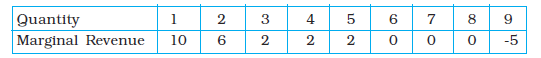
2. From the schedule provided below calculate the total revenue, demand curve and the price elasticity of demand:
3. What is the value of the MR when the demand curve is elastic?
4. A monopoly firm has a total fixed cost of Rs 100 and has the following demand schedule:
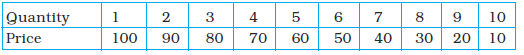
Find the short run equilibrium quantity, price and total profit. What would be the equilibrium in the long run? In case the total cost was Rs 1000, describe the equilibrium in the short run and in the long run.
5. If the monopolist firm of Exercise 3, was a public sector firm. The government set a rule for its manager to accept the goverment fixed price as given (i.e. to be a price taker and therefore behave as a firm in a perfectly competitive market), and the government decide to set the price so that demand and supply in the market are equal. What would be the equilibrium price, quantity and profit in this case?
6. Comment on the shape of the MR curve in case the TR curve is a (i) positively sloped straight line, (ii) horizontal straight line.
7. The market demand curve for a commodity and the total cost for a monopoly firm producing the commodity is given by the schedules below. Use the information to calculate the following:
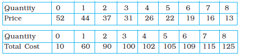
(a) The MR and MC schedules
(b) The quantites for which the MR and MC are equal
(c) The equilibrium quantity of output and the equilibrium price of the commodity
(d) The total revenue, total cost and total profit in equilibrium.
8. Will the monopolist firm continue to produce in the short run if a loss is incurred at the best short run level of output?
9. Explain why the demand curve facing a firm under monopolistic competition is negatively sloped.
10. What is the reason for the long run equilibrium of a firm in monopolistic competition to be associated with zero profit?
11. List the three different ways in which oligopoly firms may behave.
12. If duopoly behaviour is one that is described by Cournot, the market demand curve is given by the equation q = 200 – 4p, and both the firms have zero costs, find the quantity supplied by each firm in equilibrium and the equilibrium market price.
13. What is meant by prices being rigid? How can oligopoly behaviour lead to such an outcome?