Chapter 7
INTEGRALS
☘ Just as a mountaineer climbs a mountain – because it is there, so a good mathematics student studies new material because
it is there. — James B. Bristol ☘
7.1 Introduction
Differential Calculus is centred on the concept of the derivative. The original motivation for the derivative was the problem of defining tangent lines to the graphs of functions and calculating the slope of such lines. Integral Calculus is motivated by the problem of defining and calculating the area of the region bounded by the graph of the functions.
If a function f is differentiable in an interval I, i.e., its derivative f′exists at each point of I, then a natural question arises that given f′at each point of I, can we determine the function? The functions that could possibly have given function as a derivative are called anti derivatives (or primitive) of the function. Further, the formula that gives all these anti derivatives is called the indefinite integral of the function and such process of finding anti derivatives is called integration. Such type of problems arise in many practical situations. For instance, if we know the instantaneous velocity of an object at any instant, then there arises a natural question, i.e., can we determine the position of the object at any instant? There are several such practical and theoretical situations where the process of integration is involved. The development of integral calculus arises out of the efforts of solving the problems of the following types:

G .W. Leibnitz
(1646-1716)
(a) the problem of finding a function whenever its derivative is given,
(b) the problem of finding the area bounded by the graph of a function under certain conditions.
These two problems lead to the two forms of the integrals, e.g., indefinite and definite integrals, which together constitute the Integral Calculus.
There is a connection, known as the Fundamental Theorem of Calculus, between indefinite integral and definite integral which makes the definite integral as a practical tool for science and engineering. The definite integral is also used to solve many interesting problems from various disciplines like economics, finance and probability.
In this Chapter, we shall confine ourselves to the study of indefinite and definite integrals and their elementary properties including some techniques of integration.
7.2 Integration as an Inverse Process of Differentiation
Integration is the inverse process of differentiation. Instead of differentiating a function, we are given the derivative of a function and asked to find its primitive, i.e., the original function. Such a process is called integration or anti differentiation.
Let us consider the following examples:
We know that  = cos x ... (1)
 = x2 ... (2)
and  = ex ... (3)
We observe that in (1), the function cos x is the derived function of sin x. We say that sin x is an anti derivative (or an integral) of cos x. Similarly, in (2) and (3), ![]() and ex are the anti derivatives (or integrals) of x2 and ex, respectively. Again, we note that for any real number C, treated as constant function, its derivative is zero and hence, we can write (1), (2) and (3) as follows :
and ex are the anti derivatives (or integrals) of x2 and ex, respectively. Again, we note that for any real number C, treated as constant function, its derivative is zero and hence, we can write (1), (2) and (3) as follows :
 ,
,  and
and 
Thus, anti derivatives (or integrals) of the above cited functions are not unique. Actually, there exist infinitely many anti derivatives of each of these functions which can be obtained by choosing C arbitrarily from the set of real numbers. For this reason C is customarily referred to as arbitrary constant. In fact, C is the parameter by varying which one gets different anti derivatives (or integrals) of the given function. More generally, if there is a function F such that  ,
, ![]() x ∈ I (interval), then for any arbitrary real number C, (also called constant of integration)
x ∈ I (interval), then for any arbitrary real number C, (also called constant of integration)
 = f(x), x ∈ I
Thus, {F + C, C ∈ R} denotes a family of anti derivatives of f.
Remark Functions with same derivatives differ by a constant. To show this, let g and h be two functions having the same derivatives on an interval I.
Consider the function f = g – h defined by f(x) = g(x) – h(x), ![]() x ∈ I
x ∈ I
Then ![]() = f′ = g′ – h′ giving f′ (x) = g′ (x) – h′ (x)
= f′ = g′ – h′ giving f′ (x) = g′ (x) – h′ (x) ![]() x ∈ I
x ∈ I
or f′ (x) = 0, ![]() x ∈ I by hypothesis,
x ∈ I by hypothesis,
i.e., the rate of change of f with respect to x is zero on I and hence f is constant.
In view of the above remark, it is justified to infer that the family {F + C, C ∈ R} provides all possible anti derivatives of f.
We introduce a new symbol, namely, ![]() which will represent the entire class of anti derivatives read as the indefinite integral of f with respect to x.
which will represent the entire class of anti derivatives read as the indefinite integral of f with respect to x.
Symbolically, we write ![]() .
.
Notation Given that  , we write y =
 ![]() .
.
For the sake of convenience, we mention below the following symbols/terms/phrases with their meanings as given in the Table (7.1).
| Symbols/Terms/Phrases | Meaning |
| Integral of f with respect to x | |
| f(x) in |
Integrand |
| x in |
Variable of integration |
| Integrate |
Find the integral |
| An integral of f |
A function F such that F′(x) = f (x) |
| Integration |
The process of finding the integral |
| Constant of Integration |
Any real number C, considered as constant function |
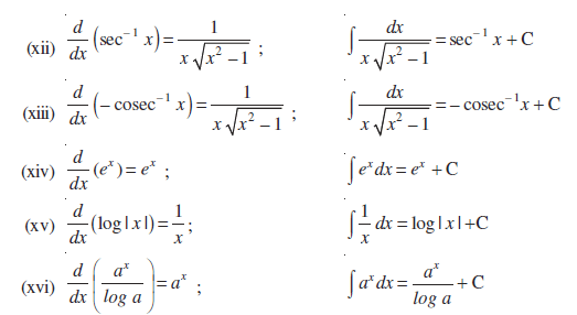
We already know the formulae for the derivatives of many important functions. From these formulae, we can write down immediately the corresponding formulae (referred to as standard formulae) for the integrals of these functions, as listed below which will be used to find integrals of other functions.
Table 7.1
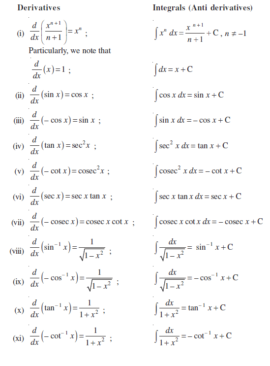
☘ Note In practice, we normally do not mention the interval over which the various functions are defined. However, in any specific problem one has to keep it in mind.
7.2.1 Geometrical interpretation of indefinite integral
Let f(x) = 2x. Then ![]() . For different values of C, we get different integrals. But these integrals are very similar geometrically.
. For different values of C, we get different integrals. But these integrals are very similar geometrically.
Thus, y = x2 + C, where C is arbitrary constant, represents a family of integrals. By assigning different values to C, we get different members of the family. These together constitute the indefinite integral. In this case, each integral represents a parabola with its axis along y-axis.
Clearly, for C = 0, we obtain y = x2, a parabola with its vertex on the origin. The curve y = x2 + 1 for C = 1 is obtained by shifting the parabola y = x2 one unit along y-axis in positive direction. For C = – 1, y = x2 – 1 is obtained by shifting the parabola y = x2 one unit along y-axis in the negative direction. Thus, for each positive value of C, each parabola of the family has its vertex on the positive side of the y-axis and for negative values of C, each has its vertex along the negative side of the y-axis. Some of these have been shown in the Fig 7.1.
Let us consider the intersection of all these parabolas by a line x = a. In the Fig 7.1, we have taken a > 0. The same is true when a < 0. If the line x = a intersects the parabolas y = x2, y = x2 + 1, y = x2 + 2, y = x2 – 1, y = x2 – 2 at P0, P1, P2, P–1, P–2 etc., respectively, then ![]() at these points equals 2a. This indicates that the tangents to the curves at these points are parallel. Thus,
at these points equals 2a. This indicates that the tangents to the curves at these points are parallel. Thus, ![]() (say), implies that the tangents to all the curves y = FC (x), C ∈ R, at the points of intersection of the curves by the line x = a, (a ∈ R), are parallel.
(say), implies that the tangents to all the curves y = FC (x), C ∈ R, at the points of intersection of the curves by the line x = a, (a ∈ R), are parallel.
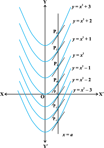
Fig 7.1
Further, the following equation (statement)![]() , represents a family of curves. The different values of C will correspond to different members of this family and these members can be obtained by shifting any one of the curves parallel to itself. This is the geometrical interpretation of indefinite integral.
, represents a family of curves. The different values of C will correspond to different members of this family and these members can be obtained by shifting any one of the curves parallel to itself. This is the geometrical interpretation of indefinite integral.
7.2.2 Some properties of indefinite integral
In this sub section, we shall derive some properties of indefinite integrals.
(I) The process of differentiation and integration are inverses of each other in the sense of the following results :
 = f(x)
and ![]() = f(x) + C, where C is any arbitrary constant.
= f(x) + C, where C is any arbitrary constant.
Proof Let F be any anti derivative of f, i.e.,
 = f(x)
Then ![]() = F(x) + C
= F(x) + C
Therefore  =
= 
= 
Similarly, we note that
f′(x) = 
and hence ![]() = f(x) + C
= f(x) + C
where C is arbitrary constant called constant of integration.
(II) Two indefinite integrals with the same derivative lead to the same family of curves and so they are equivalent.
Proof Let f and g be two functions such that
= 
or  = 0
= 0
Hence ![]() = C, where C is any real number (Why?)
= C, where C is any real number (Why?)
or ![]() =
= ![]()
So the families of curves ![]()
and ![]() are identical.
are identical.
Hence, in this sense, ![]() are equivalent.
are equivalent.
☘ Note The equivalence of the families ![]() and
and ![]() is customarily expressed by writing
is customarily expressed by writing ![]() , without mentioning the parameter.
, without mentioning the parameter.
(III) ![]()
Proof By Property (I), we have
 = f(x) + g(x) ... (1)
On the otherhand, we find that
 =
= 
= f(x) + g(x) ... (2)
Thus, in view of Property (II), it follows by (1) and (2) that
![]() =
= ![]() .
.
(IV) For any real number k, ![]()
Proof By the Property (I),  .
.
Also  =
= 
Therefore, using the Property (II), we have ![]() .
.
(V) Properties (III) and (IV) can be generalised to a finite number of functions
f1, f2, ..., fn and the real numbers, k1, k2, ..., kn giving
![]()
= ![]() .
.
To find an anti derivative of a given function, we search intuitively for a function whose derivative is the given function. The search for the requisite function for finding an anti derivative is known as integration by the method of inspection. We illustrate it through some examples.
Example 1 Write an anti derivative for each of the following functions using the method of inspection:
(i) cos 2x (ii) 3x2 + 4x3 (iii) ![]() , x ≠ 0
, x ≠ 0
Solution
(i) We look for a function whose derivative is cos 2x. Recall that
![]() sin 2x = 2 cos 2x
sin 2x = 2 cos 2x
or cos 2x =  (sin 2x) =
Therefore, an anti derivative of cos 2x is  .
.
(ii) We look for a function whose derivative is 3x2 + 4x3. Note that
 = 3x2 + 4x3.
Therefore, an anti derivative of 3x2 + 4x3 is x3 + x4.
(iii) We know that
Combining above, we get 
Therefore,  is one of the anti derivatives of
 ![]() .
.
Example 2 Find the following integrals:
(i)  (ii)
(ii)  (iii)
(iii) ![]()
Solution
(i) We have
 (by Property V)
= 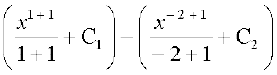 ; C1, C2 are constants of integration
= 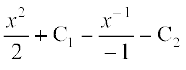 =
= 
=  , where C = C1 – C2 is another constant of integration.
☘ Note From now onwards, we shall write only one constant of integration in the final answer.
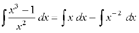
(ii) We have
=  =
= 
(iii) We have 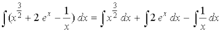
= 
= 
Example 3 Find the following integrals:
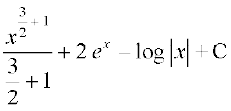
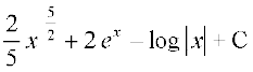
(i) ![]() (ii)
(ii) ![]()
(iii) 
Solution
(i) We have
![]()
= ![]()
(ii) We have
![]()
= ![]()
(iii) We have
= ![]()
= ![]()
Example 4 Find the anti derivative F of f defined by f (x) = 4x3 – 6, where F (0) = 3
Solution One anti derivative of f (x) is x4 – 6x since
 = 4x3 – 6
Therefore, the anti derivative F is given by
F(x) = x4 – 6x + C, where C is constant.
Given that F(0) = 3, which gives,
3 = 0 – 6 × 0 + C or C = 3
Hence, the required anti derivative is the unique function F defined by
F(x) = x4 – 6x + 3.
Remarks
(i) We see that if F is an anti derivative of f, then so is F + C, where C is any constant. Thus, if we know one anti derivative F of a function f, we can write down an infinite number of anti derivatives of f by adding any constant to F expressed by F(x) + C, C ∈ R .In applications, it is often necessary to satisfy an additional condition which then determines a specific value of C giving unique anti derivative of the given function.
(ii) Sometimes, F is not expressible in terms of elementary functions viz., polynomial, logarithmic, exponential, trigonometric functions and their inverses etc. We are therefore blocked for finding ![]() . For example, it is not possible to find
. For example, it is not possible to find ![]() by inspection since we can not find a function whose derivative is
by inspection since we can not find a function whose derivative is ![]()
(iii) When the variable of integration is denoted by a variable other than x, the integral formulae are modified accordingly. For instance
7.2.3 Comparison between differentiation and integration
1. Both are operations on functions.
2. Both satisfy the property of linearity, i.e.,
(i) 
(ii) ![]()
Here k1 and k2 are constants.
3. We have already seen that all functions are not differentiable. Similarly, all functions are not integrable. We will learn more about nondifferentiable functions and nonintegrable functions in higher classes.
4. The derivative of a function, when it exists, is a unique function. The integral of a function is not so. However, they are unique upto an additive constant, i.e., any two integrals of a function differ by a constant.
5. When a polynomial function P is differentiated, the result is a polynomial whose degree is 1 less than the degree of P. When a polynomial function P is integrated, the result is a polynomial whose degree is 1 more than that of P.
6. We can speak of the derivative at a point. We never speak of the integral at a point, we speak of the integral of a function over an interval on which the integral is defined as will be seen in Section 7.7.
7. The derivative of a function has a geometrical meaning, namely, the slope of the tangent to the corresponding curve at a point. Similarly, the indefinite integral of a function represents geometrically, a family of curves placed parallel to each other having parallel tangents at the points of intersection of the curves of the family with the lines orthogonal (perpendicular) to the axis representing the variable of integration.
8. The derivative is used for finding some physical quantities like the velocity of a moving particle, when the distance traversed at any time t is known. Similarly, the integral is used in calculating the distance traversed when the velocity at time t is known.
9. Differentiation is a process involving limits. So is integration, as will be seen in Section 7.7.
10. The process of differentiation and integration are inverses of each other as discussed in Section 7.2.2 (i).
exercise 7.1
Find an anti derivative (or integral) of the following functions by the method of inspection.
1. sin 2x
2. cos 3x
3. e2x
4. (ax + b)2
5. sin 2x – 4 e3x
Find the following integrals in Exercises 6 to 20:
6. ![]()
7. 
8. ![]()
9. ![]()
10. 
11. 
12. 
13. 
14. ![]()
15. ![]()
16. ![]()
17. ![]()
18. ![]()
19. 
20.  dx.
dx.
Choose the correct answer in Exercises 21 and 22.
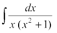
21. The anti derivative of  equals
(A) 
(B) 
(C) 
(D) 
22. If  such that f(2) = 0. Then f(x) is
(A)  (B)
(B) 
(C)  (D)
(D) 
7.3 Methods of Integration
In previous section, we discussed integrals of those functions which were readily obtainable from derivatives of some functions. It was based on inspection, i.e., on the search of a function F whose derivative is f which led us to the integral of f. However, this method, which depends on inspection, is not very suitable for many functions. Hence, we need to develop additional techniques or methods for finding the integrals by reducing them into standard forms. Prominent among them are methods based on:
1. Integration by Substitution
2. Integration using Partial Fractions
3. Integration by Parts
7.3.1 Integration by substitution
In this section, we consider the method of integration by substitution.
The given integral ![]() can be transformed into another form by changing the independent variable x to t by substituting x = g(t).
can be transformed into another form by changing the independent variable x to t by substituting x = g(t).
Consider I = ![]()
Put x = g(t) so that ![]() = g′(t).
= g′(t).
We write dx = g′(t) dt
Thus
I = ![]()
This change of variable formula is one of the important tools available to us in the name of integration by substitution. It is often important to guess what will be the useful substitution. Usually, we make a substitution for a function whose derivative also occurs in the integrand as illustrated in the following examples.
Example 5 Integrate the following functions w.r.t. x:
(i) sin mx (ii) 2x sin (x2 + 1)
(iii)  (iv)
(iv) 
Solution
(i) We know that derivative of mx is m. Thus, we make the substitution
mx = t so that mdx = dt.
Therefore,  = –
= – ![]() cos t + C = –
cos t + C = – ![]() cos mx + C
cos mx + C
(ii) Derivative of x2 + 1 is 2x. Thus, we use the substitution x2 + 1 = t so that 2x dx = dt.
Therefore, ![]() = – cos t + C = – cos (x2 + 1) + C
= – cos t + C = – cos (x2 + 1) + C
(iii) Derivative of ![]() is
is  . Thus, we use the substitution
 dx = 2t dt.
Thus, 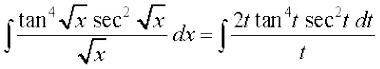 =
= ![]()
Again, we make another substitution tan t = u so that sec2 t dt = du
Therefore, ![]() =
= 
=  (since u = tan t)
= 
Hence, 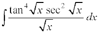 =
= 
Alternatively, make the substitution ![]()
(iv) Derivative of  . Thus, we use the substitution
tan–1 x = t so that  = dt.
= dt.
Therefore , 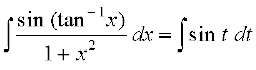 = – cos t + C = – cos(tan –1x) + C
Now, we discuss some important integrals involving trigonometric functions and their standard integrals using substitution technique. These will be used later without reference.
(i) ![]()
We have
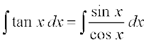
Put cos x = t so that sin x dx = – dt
Then 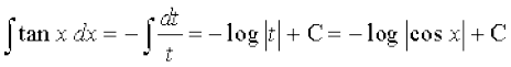
or ![]()
(ii) ![]()
We have 
Put sin x = t so that cos x dx = dt
Then  =
= ![]() =
= ![]()
(iii) ![]()
We have
Put sec x + tan x = t so that sec x (tan x + sec x) dx = dt
Therefore , 
(iv) ![]()
We have
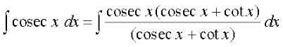
Put cosec x + cot x = t so that – cosec x (cosec x + cot x) dx = dt
So 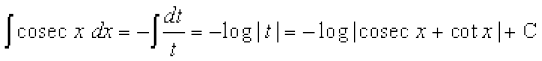
= 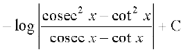
= ![]()
Example 6 Find the following integrals:
(i) ![]()
(ii) 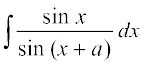
(iii) 
Solution
(i) We have
![]()
= ![]()
Put t = cos x so that dt = – sin x dx
Therefore , ![]() =
= ![]()
= 
= 
(ii) Put x + a = t. Then dx = dt. Therefore
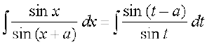
= 
= ![]()
= ![]()
= ![]()
= ![]()
Hence, = x cos a – sin a log |sin (x + a)| + C,
where, C = – C1 sin a + a cos a, is another arbitrary constant.
(iii) 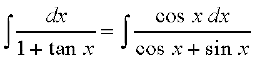
= 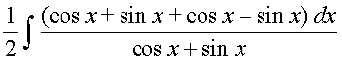
= 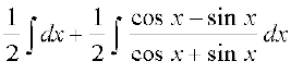
=  ... (1)
Now, consider 
Put cos x + sin x = t so that (cos x – sin x) dx = dt
Therefore  =
= ![]()
Putting it in (1), we get
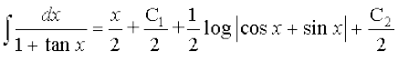
= 
= 
EXERCISE 7.2
Integrate the functions in Exercises 1 to 37:
1. 
2. 
3. 
4. ![]()
5. ![]()
6. ![]()
7. ![]()
8. ![]()
9. ![]()
10. 
11.  , x > 0
12. 
13. 
14.  , x > 0,
 ![]()
15. 
16. ![]()
17. ![]()
18. 
19. 
20. 
21. tan2 (2x – 3)
22. sec2 (7 – 4x)
23. 
24. 
25. 
26. 
27. ![]()
28. 
29. cot x log sin x
30. 
31. 
32. 
33. 
34. 
35. 
36. 
37. 
Choose the correct answer in Exercises 38 and 39.
38.  equals
(A) 10x – x10 + C
(B) 10x + x10 + C
(C) (10x – x10)–1 + C
(D) log (10x + x10) + C
39. 
(A) tan x + cot x + C
(B) tan x – cot x + C
(C) tan x cot x + C
(D) tan x – cot 2x + C
7.3.2 Integration using trigonometric identities
When the integrand involves some trigonometric functions, we use some known identities to find the integral as illustrated through the following example.
Example 7 Find (i) ![]() (ii)
(ii) ![]() (iii)
(iii) ![]()
Solution
(i) Recall the identity cos 2x = 2 cos2 x – 1, which gives
cos2x = 
Therefore , ![]() =
=  =
= 
= 
(ii) Recall the identity sin x cos y = ![]() [sin (x + y) + sin (x – y)] (Why?)
[sin (x + y) + sin (x – y)] (Why?)
Then ![]() =
= 
= 
= 
(iii) From the identity sin 3x = 3 sin x – 4 sin3 x, we find that
sin3x = 
Therefore, ![]() =
= 
= 
Alternatively, ![]() =
= ![]()
Put cos x = t so that – sin x dx = dt
Therefore, ![]() =
= ![]() =
= 
= 
Remark It can be shown using trigonometric identities that both answers are equivalent.
EXERCISE 7.3
Find the integrals of the functions in Exercises 1 to 22:
1. sin2 (2x + 5)
2. sin 3x cos 4x
3. cos 2x cos 4x cos 6x
4. sin3 (2x + 1)
5. sin3 x cos3 x
6. sin x sin 2x sin 3x
7. sin 4x sin 8x
8. 
9. 
10. sin4 x
11. cos4 2x
12. 
13. 
14. 
15. tan3 2x sec 2x
16. tan4x
17. 
18. 
19. 
20. 
21. sin – 1 (cos x)
22. 
Choose the correct answer in Exercises 23 and 24.
23. 
(A) tan x + cot x + C
(B) tan x + cosec x + C
(C) – tan x + cot x + C
(D) tan x + sec x + C
24. 
(A) – cot (exx) + C
(B) tan (xex) + C
(C) tan (ex) + C
(D) cot (ex) + C
7.4 Integrals of Some Particular Functions
In this section, we mention below some important formulae of integrals and apply them for integrating many other related standard integrals:
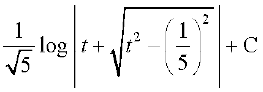
(1) 
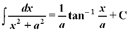
(2) 
(3) 
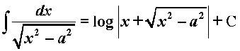
(4) 
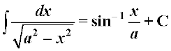
(5) 
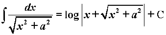
(6) 
We now prove the above results:
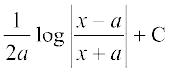
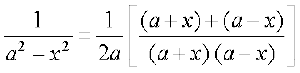
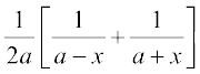
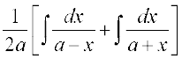
(1) We have 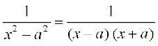
= 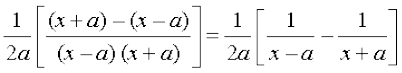
Therefore, 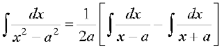
= 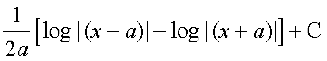
= 
(2) In view of (1) above, we have
 =
= 
Therefore,  =
= 
= 
= 
☘ Note The technique used in (1) will be explained in Section 7.5.
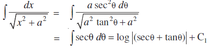
(3) Put x = a tan θ. Then dx = a sec2 θ dθ.
Therefore, 
(4) Let x = a secθ. Then dx = a secθ tanθ dθ.
Therefore, 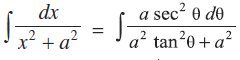
= ![]()
= 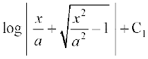
= 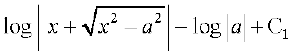
= 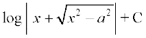 , where C = C1 – log |a|
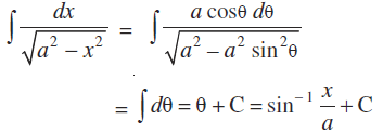
(5) Let x = a sinθ. Then dx = a cosθ dθ.
Therefore,
=
(6) Let x = a tanθ. Then dx = a sec2θ dθ.
Therefore,
= 
= 
=  , where C = C1 – log |a|
Applying these standard formulae, we now obtain some more formulae which are useful from applications point of view and can be applied directly to evaluate other integrals.
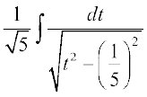
(7) To find the integral  , we write
ax2 + bx + c = 
Now, put  so that dx = dt and writing
  . We find the integral reduced to the form
  depending upon the sign of
  and hence can be evaluated.
(8) To find the integral of the type  , proceeding as in (7), we obtain the integral using the standard formulae.
(9) To find the integral of the type  , where p, q, a, b, c are constants, we are to find real numbers A, B such that
To determine A and B, we equate from both sides the coefficients of x and the constant terms. A and B are thus obtained and hence the integral is reduced to one of the known forms.
(10) For the evaluation of the integral of the type  , we proceed as in (9) and transform the integral into known standard forms.
Let us illustrate the above methods by some examples.
Example 8 Find the following integrals:
(i)  (ii)
(ii) 
Solution
(i) We have  =
=  [by 7.4 (1)]
(ii) 
Put x – 1 = t. Then dx = dt.
Therefore, =  =
= ![]() [by 7.4 (5)]
[by 7.4 (5)]
= ![]()
Example 9 Find the following integrals :
(i)  (ii)
(ii)  (iii)
(iii) 
Solution
(i) We have x2 – 6x + 13 = x2 – 6x + 32 – 32 + 13 = (x – 3)2 + 4
So,  =
= 
Let x – 3 = t. Then dx = dt
Therefore, =  [by 7.4 (3)]
= 
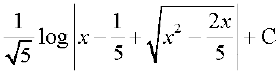
(ii) The given integral is of the form 7.4 (7). We write the denominator of the integrand,
![]() =
= 
=  (completing the square)
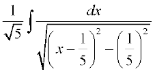
Thus  =
= 
Put  . Then dx = dt.
Therefore, = 
=  [by 7.4 (i)]
= 
= 
= 
=  , where C =
(iii) We have 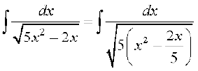
=  (completing the square)
Put  . Then dx = dt.
Therefore,  =
= 
=  [by 7.4 (4)]
= 
Example 10 Find the following integrals:
(i) 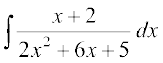 (ii)
(ii) 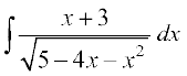
Solution
(i) Using the formula 7.4 (9), we express
x + 2 =  =
= ![]()
Equating the coefficients of x and the constant terms from both sides, we get
4A = 1 and 6A + B = 2 or A = ![]() and B =
and B = ![]() .
.
Therefore,  =
= 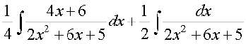
=  (say) ... (1)
In I1, put 2x2 + 6x + 5 = t, so that (4x + 6) dx = dt
Therefore, I1 = 
= ![]() ... (2)
... (2)
and I2 = 
= 
Put  , so that dx = dt, we get
I2 =  =
=  [by 7.4 (3)]
=  =
= ![]() ... (3)
... (3)
Using (2) and (3) in (1), we get
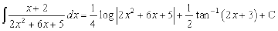
where, C = 
(ii) This integral is of the form given in 7.4 (10). Let us express
x + 3 =  = A (– 4 – 2x) + B
Equating the coefficients of x and the constant terms from both sides, we get
– 2A = 1 and – 4 A + B = 3, i.e., A = ![]() and B = 1
and B = 1
Therefore,  =
= 
= ![]() I1 + I2 ... (1)
I1 + I2 ... (1)
In I1, put 5 – 4x – x2 = t, so that (– 4 – 2x) dx = dt.
Therefore, I1=  =
= ![]()
= ![]() ... (2)
... (2)
Now consider I2 = 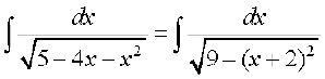
Put x + 2 = t, so that dx = dt.
Therefore, I2 = 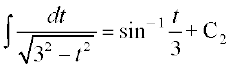 [by 7.4 (5)]
= 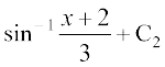 ... (3)
Substituting (2) and (3) in (1), we obtain
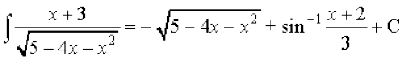 , where
EXERCISE 7.4
Integrate the functions in Exercises 1 to 23.
1. 
2. 
3. 
4. 
5. 
6. 
7. 
8. 
9. 
10. 
11. 
12. 
13. 
14. 
15. 
16. 
17. 
18. 
19. 
20. 
21. 
22. 
23.  .
.
Choose the correct answer in Exercises 24 and 25.
24. 
(A) x tan–1 (x + 1) + C
(B) tan–1 (x + 1) + C
(C) (x + 1) tan–1x + C
(D) tan–1x + C
25. 
(A) 
(B) 
(C) 
(D) 
7.5 Integration by Partial Fractions
Recall that a rational function is defined as the ratio of two polynomials in the form  , where P (x) and Q(x) are polynomials in x and Q(x) ≠ 0. If the degree of P(x) is less than the degree of Q(x), then the rational function is called proper, otherwise, it is called improper. The improper rational functions can be reduced to the proper rational functions by long division process. Thus, if is improper, then
 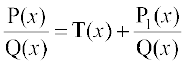 , where T(x) is a polynomial in x and
  is a proper rational function. As we know how to integrate polynomials, the integration of any rational function is reduced to the integration of a proper rational function. The rational functions which we shall consider here for integration purposes will be those whose denominators can be factorised into linear and quadratic factors. Assume that we want to evaluate
  , where is proper rational function. It is always possible to write the integrand as a sum of simpler rational functions by a method called partial fraction decomposition. After this, the integration can be carried out easily using the already known methods. The following Table 7.2 indicates the types of simpler partial fractions that are to be associated with various kind of rational functions.
Table 7.2
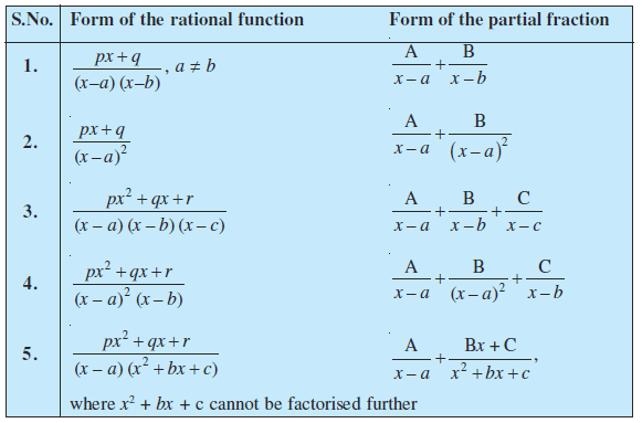
In the above table, A, B and C are real numbers to be determined suitably.
Example 11 Find 
Solution The integrand is a proper rational function. Therefore, by using the form of partial fraction [Table 7.2 (i)], we write
 =
=  ... (1)
where, real numbers A and B are to be determined suitably. This gives
1 = A (x + 2) + B (x + 1).
Equating the coefficients of x and the constant term, we get
A + B = 0
and 2A + B = 1
Solving these equations, we get A = 1 and B = – 1.
Thus, the integrand is given by
= 
Therefore, = 
= ![]()
= 
Remark The equation (1) above is an identity, i.e. a statement true for all (permissible) values of x. Some authors use the symbol ‘≡’ to indicate that the statement is an identity and use the symbol ‘=’ to indicate that the statement is an equation, i.e., to indicate that the statement is true only for certain values of x.
Example 12 Find 
Solution Here the integrand  is not proper rational function, so we divide x2 + 1 by x2 – 5x + 6 and find that
= 
Let  =
= 
So that 5x – 5 = A (x – 3) + B (x – 2)
Equating the coefficients of x and constant terms on both sides, we get A + B = 5 and 3A + 2B = 5. Solving these equations, we get A = – 5 and B = 10
Thus, = 
Therefore, 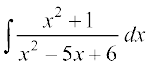 =
= 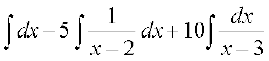
= x – 5 log |x – 2| + 10 log |x – 3| + C.
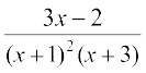
Example 13 Find 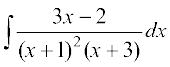
Solution The integrand is of the type as given in Table 7.2 (4). We write
 =
= 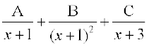
So that 3x – 2 = A (x + 1) (x + 3) + B (x + 3) + C (x + 1)2
= A (x2 + 4x + 3) + B (x + 3) + C (x2 + 2x + 1 )
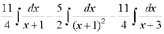
Comparing coefficient of x2, x and constant term on both sides, we get
A + C = 0, 4A + B + 2C = 3 and 3A + 3B + C = – 2. Solving these equations, we get 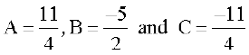 . Thus the integrand is given by
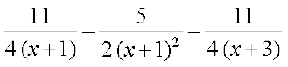
 =
= 
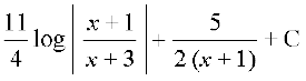
Therefore, 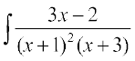 =
= 
= 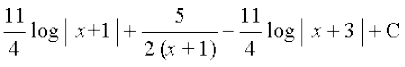
= 
Example 14 Find 
Solution Consider  and put x2 = y.
Then  =
= 
Write = 
So that y = A (y + 4) + B (y + 1)
Comparing coefficients of y and constant terms on both sides, we get A + B = 1 and 4A + B = 0, which give
A = 
Thus, = 
Therefore, 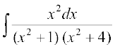 =
= 
= 
= 
In the above example, the substitution was made only for the partial fraction part and not for the integration part. Now, we consider an example, where the integration involves a combination of the substitution method and the partial fraction method.
Example 15 Find 
Solution Let y = sinφ
Then dy = cosφ dφ
Therefore,  =
= 
= 
= 
Now, we write  =
=  [by Table 7.2 (2)]
Therefore, 3y – 2 = A (y – 2) + B
Comparing the coefficients of y and constant term, we get A = 3 and B – 2A = – 2, which gives A = 3 and B = 4.
Therefore, the required integral is given by
I =  =
= 
= 
= 
=  (since, 2 – sinφ is always positive)
Example 16 Find 
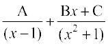
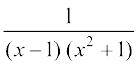
Solution The integrand is a proper rational function. Decompose the rational function into partial fraction [Table 2.2(5)]. Write
 =
= 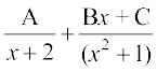
Therefore, x2 + x + 1 = A (x2 + 1) + (Bx + C) (x + 2)
Equating the coefficients of x2, x and of constant term of both sides, we get
A + B =1, 2B + C = 1 and A + 2C = 1. Solving these equations, we get 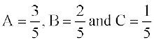
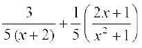
Thus, the integrand is given by
= 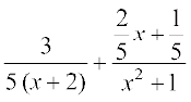 =
= 
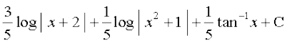
Therefore, 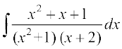 =
= 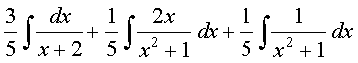
= 
EXERCISE 7.5
Integrate the rational functions in Exercises 1 to 21.
1. 
2. 
3. 
4. 
5. 
6. 
7. 
8. 
9. 
10. 
11. 
12. 
13. 
14. 
15. 
16.  [Hint: multiply numerator and denominator by x n – 1 and put xn = t ]
17.  [Hint : Put sin x = t]
18. 
19. 
20. 
21.  [Hint : Put ex = t]
Choose the correct answer in each of the Exercises 22 and 23.
22. 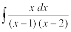 equals
(A) 
(B) 
(C) 
(D) ![]()
23.  equals
(A) 
(B) 
(C) 
(D) 
7.6 Integration by Parts
In this section, we describe one more method of integration, that is found quite useful in integrating products of functions.
If u and v are any two differentiable functions of a single variable x (say). Then, by the product rule of differentiation, we have
 =
= 
Integrating both sides, we get
uv = 
or  =
=  ... (1)
Let u = f(x) and ![]() = g(x). Then
= g(x). Then
![]() = f′(x) and v =
= f′(x) and v = ![]()
Therefore, expression (1) can be rewritten as
![]() =
= ![]()
i.e., ![]() =
= ![]()
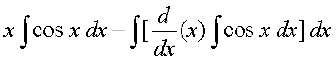
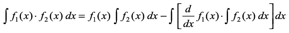
If we take f as the first function and g as the second function, then this formula may be stated as follows:
“The integral of the product of two functions = (first function) × (integral of the second function) – Integral of [(differential coefficient of the first function) × (integral of the second function)]”
Example 17 Find ![]()
Solution Put f (x) = x (first function) and g (x) = cos x (second function).
Then, integration by parts gives
![]() =
= 
= ![]() = x sin x + cos x + C
= x sin x + cos x + C
Suppose, we take f(x) = cos x and g(x) = x. Then
![]() =
= 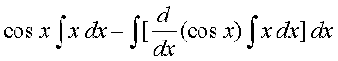
= 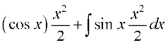
Thus, it shows that the integral ![]() is reduced to the comparatively more complicated integral having more power of x. Therefore, the proper choice of the first function and the second function is significant.
is reduced to the comparatively more complicated integral having more power of x. Therefore, the proper choice of the first function and the second function is significant.
Remarks
(i) It is worth mentioning that integration by parts is not applicable to product of functions in all cases. For instance, the method does not work for ![]() . The reason is that there does not exist any function whose derivative is
. The reason is that there does not exist any function whose derivative is ![]() sin x.
sin x.
(ii) Observe that while finding the integral of the second function, we did not add any constant of integration. If we write the integral of the second function cos x as sin x + k, where k is any constant, then
![]() =
= ![]()
= ![]()
= ![]() =
= ![]()
This shows that adding a constant to the integral of the second function is superfluous so far as the final result is concerned while applying the method of integration by parts.
(iii) Usually, if any function is a power of x or a polynomial in x, then we take it as the first function. However, in cases where other function is inverse trigonometric function or logarithmic function, then we take them as first function.
Example 18 Find ![]()
Solution To start with, we are unable to guess a function whose derivative is log x. We take log x as the first function and the constant function 1 as the second function. Then, the integral of the second function is x.
Hence, ![]() =
= 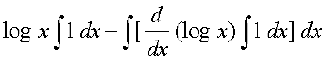
= 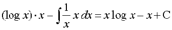 .
.
Example 19 Find ![]()
Solution Take first function as x and second function as ex. The integral of the second function is ex.
Therefore, ![]() =
= ![]() = xex – ex + C.
= xex – ex + C.
Example 20 Find 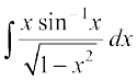
Solution Let first function be sin – 1x and second function be  .
.
First we find the integral of the second function, i.e.,  .
.
Put t =1 – x2. Then dt = – 2x dx
Therefore, =  =
= ![]()
Hence, 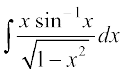 =
= 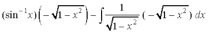
= ![]() =
= ![]()
Alternatively, this integral can also be worked out by making substitution sin–1 x = θ and then integrating by parts.
Example 21 Find ![]()
Solution Take ex as the first function and sin x as second function. Then, integrating by parts, we have
![]()
= – ex cos x + I1 (say) ... (1)
Taking ex and cos x as the first and second functions, respectively, in I1, we get
I1 = ![]()
Substituting the value of I1 in (1), we get
I = – ex cos x + ex sin x – I or 2I = ex (sin x – cos x)
Hence, I = 
Alternatively, above integral can also be determined by taking sin x as the first function and ex the second function.
7.6.1 Integral of the type 
We have I = ![]() =
= ![]()
= ![]() ... (1)
... (1)
Taking f(x) and ex as the first function and second function, respectively, in I1 and integrating it by parts, we have I1 = f (x) ex – ![]()
Substituting I1 in (1), we get
I = ![]() = ex f (x) + C
= ex f (x) + C
Thus, ![]() =
= ![]()
Example 22 Find (i)  dx (ii)
  dx
dx
Solution
(i) We have I =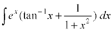
Consider f(x) = tan– 1x, then f′(x) = 
Thus, the given integrand is of the form ex [f (x) + f ′(x)].
Therefore, 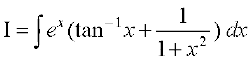 = ex tan– 1x + C
(ii) We have 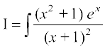 dx
dx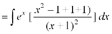
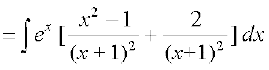
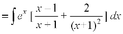
Consider 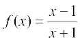 , then
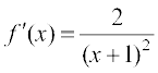
Thus, the given integrand is of the form ex [f (x) + f ′(x)].
Therefore, 
EXERCISE 7.6
Integrate the functions in Exercises 1 to 22.
1. x sin x
2. x sin 3x
3. x2 ex
4. x log x
5. x log 2x
6. x2 log x
7. x sin– 1x
8. x tan–1 x
9. x cos–1 x
10. (sin–1x)2
11. 
12. x sec2 x
13. tan–1x
14. x (log x)2
15. (x2 + 1) log x
16. ex (sinx + cosx)
17. 
18. 
19. 
20. 
21. e2x sin x
22. 
Choose the correct answer in Exercises 23 and 24.
23. ![]() equals
equals
(A) 
(B) 
(C) 
(D) 
24. ![]() equals
equals
(A) ex cos x + C
(B) ex sec x + C
(C) ex sin x + C
(D) ex tan x + C
7.6.2 Integrals of some more types
Here, we discuss some special types of standard integrals based on the technique of integration by parts :
(i) ![]() (ii)
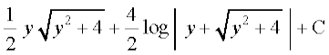
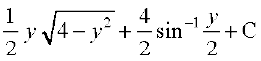
(ii) ![]() (iii)
(iii) ![]()
(i) Let ![]()
Taking constant function 1 as the second function and integrating by parts, we have
I = 
=  =
= 
= 
= 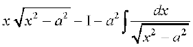
or 2I = 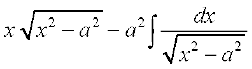
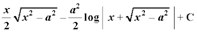
or I = ![]() =
= 
Similarly, integrating other two integrals by parts, taking constant function 1 as the second function, we get
(ii) 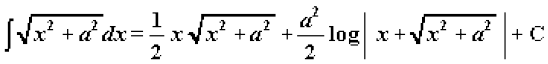
(iii) 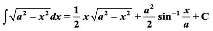
Alternatively, integrals (i), (ii) and (iii) can also be found by making trigonometric substitution x = a secθ in (i), x = a tanθ in (ii) and x = a sinθ in (iii) respectively.
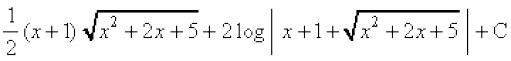
Example 23 Find ![]()
Solution Note that
![]() =
= ![]()
Put x + 1 = y, so that dx = dy. Then
![]() =
= ![]()
=  [using 7.6.2 (ii)]
= 
Example 24 Find ![]()
Solution Note that ![]()
Put x + 1 = y so that dx = dy.
Thus ![]() =
= ![]()
=  [using 7.6.2 (iii)]
= 
EXERCISE 7.7
Integrate the functions in Exercises 1 to 9.
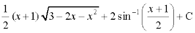
1. ![]()
2. ![]()
3. ![]()
4. ![]()
5. ![]()
6. ![]()
7. ![]()
8. ![]()
9. 
Choose the correct answer in Exercises 10 to 11.
10. ![]() is equal to
is equal to
(A) 
(B) 
(C) 
(D) 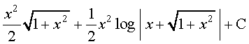
11. ![]() is equal to
is equal to
(A) 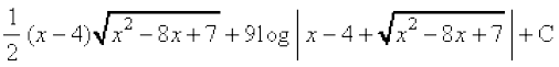
(B) 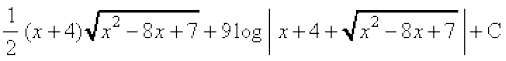
(C) 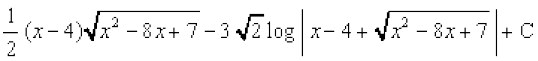
(D) 
7.7 Definite Integral
In the previous sections, we have studied about the indefinite integrals and discussed few methods of finding them including integrals of some special functions. In this section, we shall study what is called definite integral of a function. The definite integral has a unique value. A definite integral is denoted by  , where a is called the lower limit of the integral and b is called the upper limit of the integral. The definite integral is introduced either as the limit of a sum or if it has an anti derivative F in the interval [a, b], then its value is the difference between the values of F at the end points, i.e., F(b) – F(a). Here, we shall consider these two cases separately as discussed below:
7.7.1 Definite integral as the limit of a sum
Let f be a continuous function defined on close interval [a, b]. Assume that all the values taken by the function are non negative, so the graph of the function is a curve above the x-axis.
The definite integral is the area bounded by the curve y = f(x), the ordinates x = a, x = b and the x-axis. To evaluate this area, consider the region PRSQP between this curve, x-axis and the ordinates x = a and x = b (Fig 7.2).
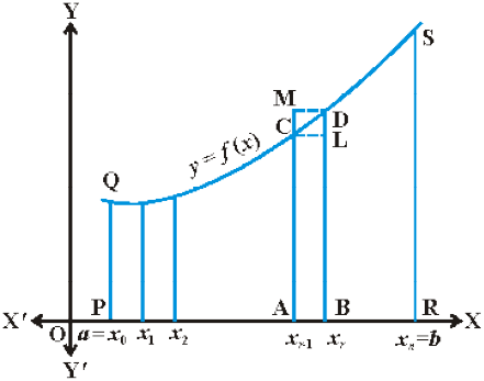
Fig 7.2
Divide the interval [a, b] into n equal subintervals denoted by [x0, x1], [x1, x2] ,..., [xr – 1, xr], ..., [xn – 1, xn], where x0 = a, x1 = a + h, x2 = a + 2h, ... , xr = a + rh and
xn = b = a + nh or  We note that as n → ∞, h → 0.
The region PRSQP under consideration is the sum of n subregions, where each subregion is defined on subintervals [xr – 1, xr], r = 1, 2, 3, …, n.
From Fig 7.2, we have
area of the rectangle (ABLC) < area of the region (ABDCA) < area of the rectangle (ABDM) ... (1)
Evidently as xr – xr–1 → 0, i.e., h → 0 all the three areas shown in (1) become nearly equal to each other. Now we form the following sums.
sn = h [f(x0) + … + f(xn - 1)] =  ... (2)
and Sn = 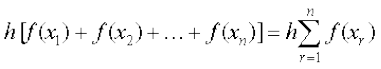 ... (3)
Here, sn and Sn denote the sum of areas of all lower rectangles and upper rectangles raised over subintervals [xr–1, xr] for r = 1, 2, 3, …, n, respectively.
In view of the inequality (1) for an arbitrary subinterval [xr–1, xr], we have
sn < area of the region PRSQP < Sn ... (4)
As![]() strips become narrower and narrower, it is assumed that the limiting values of (2) and (3) are the same in both cases and the common limiting value is the required area under the curve.
strips become narrower and narrower, it is assumed that the limiting values of (2) and (3) are the same in both cases and the common limiting value is the required area under the curve.
Symbolically, we write
![]() =
= ![]() = area of the region PRSQP =
= area of the region PRSQP =  ... (5)
It follows that this area is also the limiting value of any area which is between that
of the rectangles below the curve and that of the rectangles above the curve. For
the sake of convenience, we shall take rectangles with height equal to that of the
curve at the left hand edge of each subinterval. Thus, we rewrite (5) as
 =
= ![]()
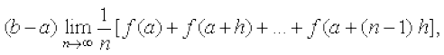
or = 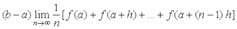 ... (6)
where h = 
The above expression (6) is known as the definition of definite integral as the limit of sum.
Remark The value of the definite integral of a function over any particular interval depends on the function and the interval, but not on the variable of integration that we choose to represent the independent variable. If the independent variable is denoted by t or u instead of x, we simply write the integral as  or
or  instead of
  . Hence, the variable of integration is called a dummy variable.
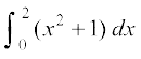
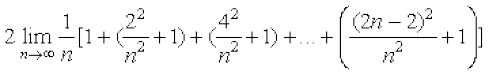
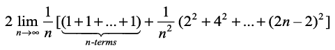
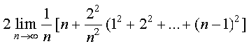
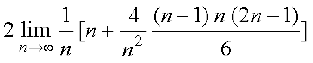
Example 25 Find  as the limit of a sum.
Solution By definition
= 
where, h = 
In this example, a = 0, b = 2, f (x) = x2 + 1, 
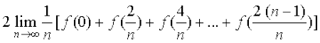
Therefore,
 =
= 
= 
= 
= 
= 
= 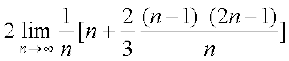
= 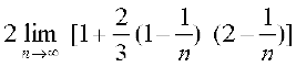 =
=  =
= ![]()
Example 26 Evaluate  as the limit of a sum.
Solution By definition
= 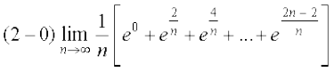
Using the sum to n terms of a G.P., where a = 1,  , we have
= 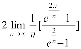 =
= 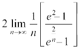
= 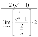 = e2 – 1 [using
 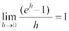 ]
]
EXERCISE 7.8
Evaluate the following definite integrals as limit of sums.
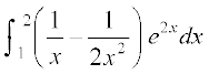
1. 
2. 
3. 
4. 
5. 
6. 
7.8 Fundamental Theorem of Calculus
7.8.1 Area function
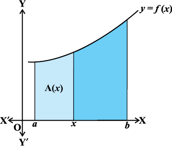
Fig 7.3
We have defined as the area of the region bounded by the curve y = f(x),
the ordinates x = a and x = b and x-axis. Let x
be a given point in [a, b]. Then  represents the area of the light shaded region
in Fig 7.3 [Here it is assumed that f(x) > 0 for x ∈ [a, b], the assertion made below is equally true for other functions as well]. The area of this shaded region depends upon the value of x.
In other words, the area of this shaded region is a function of x. We denote this function of x by A(x). We call the function A(x) as Area function and is given by
A(x) =  ... (1)
Based on this definition, the two basic fundamental theorems have been given. However, we only state them as their proofs are beyond the scope of this text book.
7.8.2 First fundamental theorem of integral calculus
Theorem 1 Let f be a continuous function on the closed interval [a, b] and let A (x) be the area function. Then A′(x) = f (x), for all x ∈ [a, b].
7.8.3 Second fundamental theorem of integral calculus
We state below an important theorem which enables us to evaluate definite integrals by making use of anti derivative.
Theorem 2 Let f be continuous function defined on the closed interval [a, b] and F be an anti derivative of f. Then  =
= ![]() F (b) – F(a).
F (b) – F(a).
Remarks
(i) In words, the Theorem 2 tells us that = (value of the anti derivative F of f at the upper limit b – value of the same anti derivative at the lower limit a).
(ii) This theorem is very useful, because it gives us a method of calculating the definite integral more easily, without calculating the limit of a sum.
(iii) The crucial operation in evaluating a definite integral is that of finding a function whose derivative is equal to the integrand. This strengthens the relationship between differentiation and integration.
(iv) In , the function f needs to be well defined and continuous in [a, b]. For instance, the consideration of definite integral  is erroneous since the function f expressed by f(x) =
  is not defined in a portion
– 1 < x < 1 of the closed interval [– 2, 3].
Steps for calculating .
(i) Find the indefinite integral![]() . Let this be F(x). There is no need to keep integration constant C because if we consider F(x) + C instead of F(x), we get
. Let this be F(x). There is no need to keep integration constant C because if we consider F(x) + C instead of F(x), we get
 .
.
Thus, the arbitrary constant disappears in evaluating the value of the definite integral.
(ii) Evaluate F(b) – F(a) = ![]() , which is the value of .
, which is the value of .
We now consider some examples
Example 27 Evaluate the following integrals:
(i) (ii) 
(iii)  (iv)
(iv) 
Solution
(i) Let  . Since
  ,
,
Therefore, by the second fundamental theorem, we get
I = 
(ii) Let 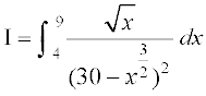 . We first find the anti derivative of the integrand.
Put  or
or 
Thus,  =
=  =
= 
Therefore, by the second fundamental theorem of calculus, we have
I = 
=  =
= 
(iii) Let 
Using partial fraction, we get 
So  =
= ![]()
Therefore, by the second fundamental theorem of calculus, we have
I = F(2) – F(1) = [– log 3 + 2 log 4] – [– log 2 + 2 log 3]
= – 3 log 3 + log 2 + 2 log 4 = 
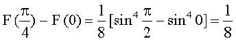
(iv) Let  . Consider
 ![]()
Put sin 2t = u so that 2 cos 2t dt = du or cos 2t dt = ![]() du
du
So ![]() =
= 
= 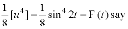
Therefore, by the second fundamental theorem of integral calculus
EXERCISE 7.9
Evaluate the definite integrals in Exercises 1 to 20.
1. 
2. 
3. 
4. ![]()
5. 
6. 
7. 
8. 
9. 
10. 
11. 
12. 
13. 
14. 
15. 
16. 
17. 
18. 
19. 
20. 
Choose the correct answer in Exercises 21 and 22.
21.  equals
(A) ![]() (B)
(B) ![]()
(C) ![]() (D)
(D) ![]()
22.  equals
(A) ![]()
(B) ![]()
(C) ![]()
(D) ![]()
7.9 Evaluation of Definite Integrals by Substitution
In the previous sections, we have discussed several methods for finding the indefinite integral. One of the important methods for finding the indefinite integral is the method of substitution.
To evaluate , by substitution, the steps could be as follows:
1. Consider the integral without limits and substitute, y = f(x) or x = g(y) to reduce the given integral to a known form.
2. Integrate the new integrand with respect to the new variable without mentioning the constant of integration.
3. Resubstitute for the new variable and write the answer in terms of the original variable.
4. Find the values of answers obtained in (3) at the given limits of integral and find the difference of the values at the upper and lower limits.
☘ Note In order to quicken this method, we can proceed as follows: After performing steps 1, and 2, there is no need of step 3. Here, the integral will be kept in the new variable itself, and the limits of the integral will accordingly be changed, so that we can perform the last step.
Let us illustrate this by examples.
Example 28 Evaluate  .
.
Solution Put t = x5 + 1, then dt = 5x4 dx.
Therefore, ![]() =
= ![]() =
= ![]() =
= 
Hence, = 
= 
=  =
= 
Alternatively, first we transform the integral and then evaluate the transformed integral with new limits.
Let t = x5 + 1. Then dt = 5 x4 dx.
Note that, when x = – 1, t = 0 and when x = 1, t = 2
Thus, as x varies from – 1 to 1, t varies from 0 to 2
Therefore = 
=  =
= 
Example 29 Evaluate 
Solution Let t = tan– 1x, then  . The new limits are, when x = 0, t = 0 and when x = 1,
  . Thus, as x varies from 0 to 1, t varies from 0 to
 ![]() .
.
Therefore  =
=  =
= 
EXERCISE 7.10
Evaluate the integrals in Exercises 1 to 8 using substitution.
1. 
2. 
3. 
4.  (Put x + 2 = t2)
5. 
6. 
7. 
8. 
Choose the correct answer in Exercises 9 and 10.
9. The value of the integral 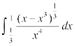 is
is
(A) 6
(B) 0
(C) 3
(D) 4
10. If f(x) = 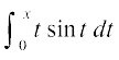 , then f′(x) is
(A) cosx + x sin x
(B) x sinx
(C) x cosx
(D) sinx + x cosx
7.10 Some Properties of Definite Integrals
We list below some important properties of definite integrals. These will be useful in evaluating the definite integrals more easily.
P0 : 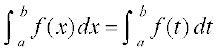
P1 :  . In particular,
P2 : 
P3 : 
P4 : 
(Note that P4 is a particular case of P3)
P5 : 
P6 :  and 0 if f(2a – x) = – f(x)
P7 : (i)  , if f is an even function, i.e., if f(– x) = f(x).
(ii)  , if f is an odd function, i.e., if f(– x) = – f(x).
We give the proofs of these properties one by one.
Proof of P0 It follows directly by making the substitution x = t.
Proof of P1 Let F be anti derivative of f. Then, by the second fundamental theorem of calculus, we have 
Here, we observe that, if a = b, then  .
.
Proof of P2 Let F be anti derivative of f. Then
= F(b) – F(a) ... (1)
 = F(c) – F(a) ... (2)
and  = F(b) – F(c) ... (3)
Adding (2) and (3), we get 
This proves the property P2.
Proof of P3 Let t = a + b – x. Then dt = – dx. When x = a, t = b and when x = b, t = a. Therefore
= 
=  (by P1)
=  dx by P0
Proof of P4 Put t = a – x. Then dt = – dx. When x = 0, t = a and when x = a, t = 0. Now proceed as in P3.
Proof of P5 Using P2, we have  .
.
Let t = 2a – x in the second integral on the right hand side. Then
dt = – dx. When x = a, t = a and when x = 2a, t = 0. Also x = 2a – t.
Therefore, the second integral becomes
 =
=  =
=  =
= 
Hence  =
= 
Proof of P6 Using P5, we have  ... (1)
Now, if f(2a – x) = f(x), then (1) becomes
= 
and if f(2a – x) = – f(x), then (1) becomes
= 
Proof of P7 Using P2, we have
 =
=  . Then
Let t = – x in the first integral on the right hand side.
dt = – dx. When x = – a, t = a and when
x = 0, t = 0. Also x = – t.
Therefore = 
=  (by P0) ... (1)
(i) Now, if f is an even function, then f(–x) = f(x) and so (1) becomes
(ii) If f is an odd function, then f(–x) = – f(x) and so (1) becomes
Example 30 Evaluate 
Solution We note that x3 – x ≥ 0 on [– 1, 0] and x3 – x ≤ 0 on [0, 1] and that
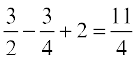
x3 – x ≥ 0 on [1, 2]. So by P2 we write
= 
= 
= 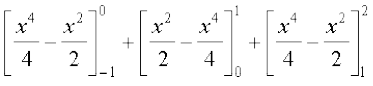
= 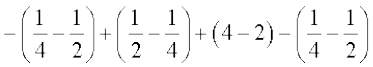
= 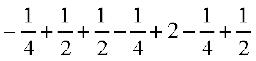 =
= 
Example 31 Evaluate 
Solution We observe that sin2 x is an even function. Therefore, by P7 (i), we get
 =
= 
=  =
= 
=  =
= 
Example 32 Evaluate 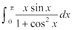
Solution Let I =  . Then, by P4, we have
I = 
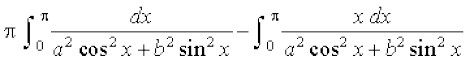
=  =
= 
or 2 I = 
or I = 
Put cos x = t so that – sin x dx = dt. When x = 0, t = 1 and when x = π, t = – 1. Therefore, (by P1) we get
I =  =
= 
=  (by P7,
  is even function)
= 
Example 33 Evaluate 
Solution Let I =  . Let f(x) = sin5 x cos4 x. Then
f(– x) = sin5 (– x) cos4 (– x) = – sin5 x cos4 x = – f(x), i.e., f is an odd function. Therefore, by P7 (ii), I = 0
Example 34 Evaluate 
Solution Let I = ... (1)
Then, by P4
I =  =
=  ... (2)
Adding (1) and (2), we get
2I = 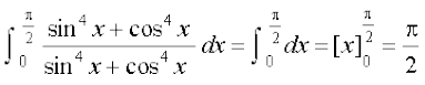
Hence I = ![]()
Example 35 Evaluate 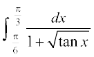
Solution Let I = 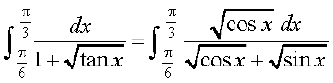 ... (1)
Then, by P3 I = 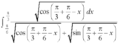
=  ... (2)
Adding (1) and (2), we get
2I =  . Hence
Example 36 Evaluate 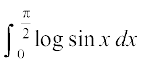
Solution Let I =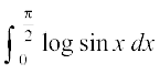
Then, by P4
I = 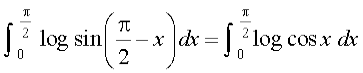
Adding the two values of I, we get
2I = 
=  (by adding and subtracting log2)
=  (Why?)
Put 2x = t in the first integral. Then 2 dx = dt, when x = 0, t = 0 and when  , t = π.
Therefore 2I = 
=  [by P6 as sin (π – t) = sin t)
=  (by changing variable t to x)
= 
Hence  =
=  .
.
EXERCISE 7.11
By using the properties of definite integrals, evaluate the integrals in Exercises 1 to 19.
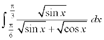
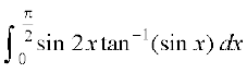
1. 
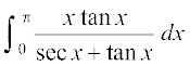
2. 
3. 
4. 
5. 
6. 
7. 
8. 
9. 
10. 
11. 
12. 
13. 
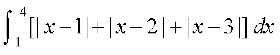
14. 
15. 
16. 
17. 
18. 
19. Show that  , if f and g are defined as f(x) = f(a – x) and g(x) + g(a – x) = 4
Choose the correct answer in Exercises 20 and 21.
20. The value of  is
is
(A) 0
(B) 2
(C) π
(D) 1
21. The value of  is
is
(A) 2
(B) ![]()
(C) 0
(D) –2
Miscellaneous Examples
Example 37 Find ![]()
Solution Put t = 1 + sin 6x, so that dt = 6 cos 6x dx
Therefore 
= 
Example 38 Find 
Solution We have 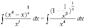
Put 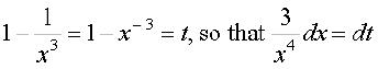
Therefore 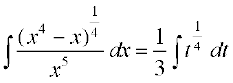 =
= 
Example 39 Find 
Solution We have
 =
= 
=  ... (1)
Now express 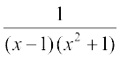 =
=  ... (2)
So 1 = A (x2 + 1) + (Bx + C) (x – 1)
= (A + B) x2 + (C – B) x + A – C
Equating coefficients on both sides, we get A + B = 0, C – B = 0 and A – C = 1, which give 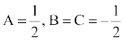 . Substituting values of A, B and C in (2), we get
 =
=  ... (3)
Again, substituting (3) in (1), we have
 =
= 
Therefore

Example 40 Find 
Solution Let 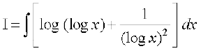
= 
In the first integral, let us take 1 as the second function. Then integrating it by parts, we get
I = 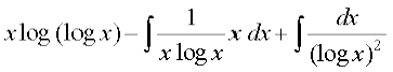
=  ... (1)
Again, consider  , take 1 as the second function and integrate it by parts,
we have 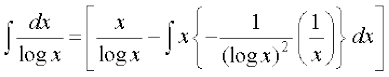 ... (2)
Putting (2) in (1), we get
 =
= 
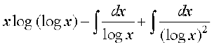
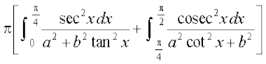
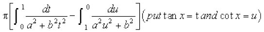
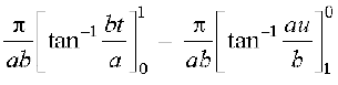
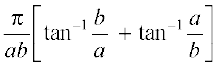
Example 41 Find ![]()
Solution We have
I = ![]()
![]()
Put tan x = t2, so that sec2 x dx = 2t dt
or dx = 
Then I = 
= 
Put ![]() = y, so that
= y, so that  dt = dy. Then
I = 
= 
Example 42 Find 
Solution Let 
Put cos2 (2x) = t so that 4 sin 2x cos 2x dx = – dt
Therefore 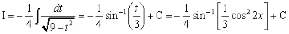
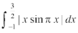
Example 43 Evaluate 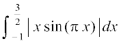
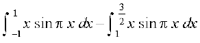
Solution Here f(x) = |x sin πx | = 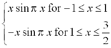
Therefore 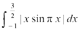 =
= 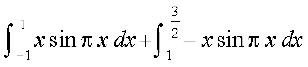
= 
Integrating both integrals on righthand side, we get
 =
= 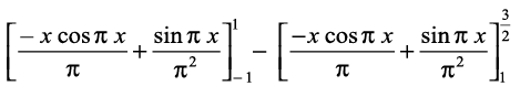
= 
Example 44 Evaluate 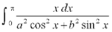
Solution Let I = 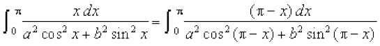 (using P4)
= 
= 
Thus 2I = 
or I =  (using P6)
= 
= 
= 
=  =
=  =
= ![]()
Miscellaneous Exercise on Chapter 7
Integrate the functions in Exercises 1 to 24.
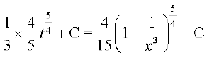
1. 
2. 
3.  [Hint: Put x =
 ![]() ]
]
4. 
5.  [Hint:
 , put x = t6]
6. 
7. 
8. 
9. 
10. 
11. 
12. 
13. 
14. 
15. cos3x elog sinx
16. e3 logx (x4 + 1)– 1
17. f′ (ax + b) [f(ax + b)]n
18. 
19.  , x ∈ [0, 1]
20. 
21. 
22. 
23.  24.
24. 
Evaluate the definite integrals in Exercises 25 to 33.
25. 
26. 
27. 
28. 
29. 
30. 
31. 
32. 
33. 
Prove the following (Exercises 34 to 39)
34.  35.
35. 
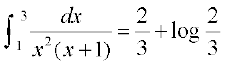
36.  37.
37. 
38.  39.
39. 
40. Evaluate  as a limit of a sum.
Choose the correct answers in Exercises 41 to 44.
41.  is equal to
(A) tan–1 (ex) + C
(B) tan–1 (e–x) + C
(C) log (ex – e–x) + C
(D) log (ex + e–x) + C
42.  is equal to
(A) 
(B) ![]()
(C) ![]()
(D) 
43. If f (a + b – x) = f (x), then  is equal to
(A) 
(B) 
(C) 
(D) 
44. The value of  is
is
(A) 1
(B) 0
(C) –1
(D) ![]()
Summary
Integration is the inverse process of differentiation. In the differential calculus, we are given a function and we have to find the derivative or differential of this function, but in the integral calculus, we are to find a function whose differential is given. Thus, integration is a process which is the inverse of differentiation.
Let  . Then we write
 ![]() . These integrals are called indefinite integrals or general integrals, C is called constant of integration. All these integrals differ by a constant.
. These integrals are called indefinite integrals or general integrals, C is called constant of integration. All these integrals differ by a constant.
From the geometric point of view, an indefinite integral is collection of family of curves, each of which is obtained by translating one of the curves parallel to itself upwards or downwards along the y-axis.
Some properties of indefinite integrals are as follows:
1. ![]()
2. For any real number k, ![]()
More generally, if f1, f2, f3, ... , fn are functions and k1, k2, ... ,kn are real numbers. Then
![]()
= ![]()
Some standard integrals
(i)  , n ≠ – 1. Particularly,
 ![]()
(ii) ![]() (iii)
(iii) ![]()
(iv) ![]() (v)
(v) ![]()
(vi) ![]()
(vii) ![]() (viii)
(viii) 
(ix)  (x)
(x) 
(xi)  (xii)
(xii) ![]()
(xiii)  (xiv)
(xiv) 
(xv)  (xvi)
(xvi) 
Integration by partial fractions
Recall that a rational function is ratio of two polynomials of the form  , where P(x) and Q(x) are polynomials in x and Q(x) ≠ 0. If degree of the polynomial P(x) is greater than the degree of the polynomial Q(x), then we may divide P(x) by Q(x) so that
 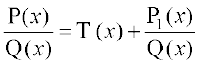 , where T(x) is a polynomial in x and degree of P1(x) is less than the degree of Q(x). T(x) being polynomial can be easily integrated.
  can be integrated by expressing
  as the sum of partial fractions of the following type:
1.  =
= 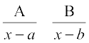 , a ≠ b
2.  =
= 
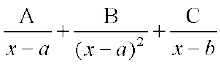
3.  =
= 
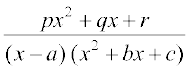
4.  =
= 
5.  =
= 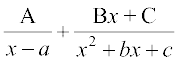
where x2 + bx + c can not be factorised further.
Integration by substitution
A change in the variable of integration often reduces an integral to one of the fundamental integrals. The method in which we change the variable to some other variable is called the method of substitution. When the integrand involves some trigonometric functions, we use some well known identities to find the integrals. Using substitution technique, we obtain the following standard integrals.
(i) ![]() (ii)
(ii) ![]()
(iii) ![]()
(iv) ![]()
Integrals of some special functions
(i) 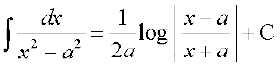
(ii) 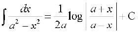 (iii)
(iii) 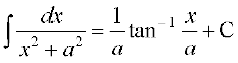
(iv) 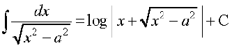 (v)
(v) 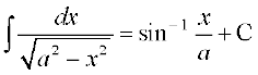
(vi) 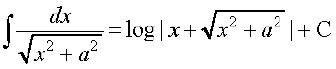
Integration by parts
For given functions f1 and f2, we have
 , i.e., the integral of the product of two functions = first function × integral of the second function – integral of {differential coefficient of the first function × integral of the second function}. Care must be taken in choosing the first function and the second function. Obviously, we must take that function as the second function whose integral is well known to us.
![]()
Some special types of integrals
(i) 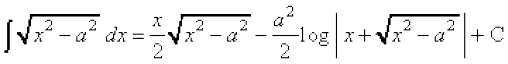
(ii) 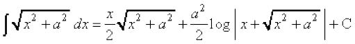
(iii) 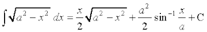
(iv) Integrals of the types 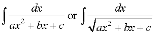 can be transformed into standard form by expressing
ax2 + bx + c = 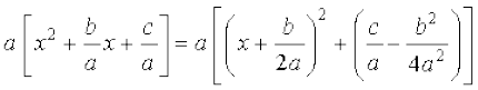
(v) Integrals of the types 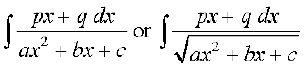 can be transformed into standard form by expressing
 , where A and B are determined by comparing coefficients on both sides.
We have defined as the area of the region bounded by the curve
y = f(x), a ≤ x ≤ b, the x-axis and the ordinates x = a and x = b. Let x be a given point in [a, b]. Then represents the Area function A(x). This concept of area function leads to the Fundamental Theorems of Integral Calculus.
First fundamental theorem of integral calculus
Let the area function be defined by A(x) = for all x ≥ a, where the function f is assumed to be continuous on [a, b]. Then A′(x) = f(x) for all x ∈ [a, b].
Let f be a continuous function of x defined on the closed interval [a, b] and let F be another function such that for all x in the domain of f, then  .
.
This is called the definite integral of f over the range [a, b], where a and b are called the limits of integration, a being the lower limit and b the
upper limit.