Chapter 12
Linear Programming
![]() The mathematical experience of the student is incomplete if he never had the opportunity to solve a problem invented by himself. – G. POLYA
The mathematical experience of the student is incomplete if he never had the opportunity to solve a problem invented by himself. – G. POLYA ![]()
12.1 Introduction

L. Kantorovich
In earlier classes, we have discussed systems of linear equations and their applications in day to day problems. In Class XI, we have studied linear inequalities and systems of linear inequalities in two variables and their solutions by graphical method. Many applications in mathematics involve systems of inequalities/equations. In this chapter, we shall apply the systems of linear inequalities/equations to solve some real life problems of the type as given below:
Such type of problems which seek to maximise (or, minimise) profit (or, cost) form a general class of problems called optimisation problems. Thus, an optimisation problem may involve finding maximum profit, minimum cost, or minimum use of resources etc.
A special but a very important class of optimisation problems is linear programming problem. The above stated optimisation problem is an example of linear programming
problem. Linear programming problems are of much interest because of their wide applicability in industry, commerce, management science etc.
In this chapter, we shall study some linear programming problems and their solutions by graphical method only, though there are many other methods also to solve such problems.
12.2 Linear Programming Problem and its Mathematical Formulation
We begin our discussion with the above example of furniture dealer which will further lead to a mathematical formulation of the problem in two variables. In this example, we observe
(i) The dealer can invest his money in buying tables or chairs or combination thereof. Further he would earn different profits by following different investment strategies.
(ii) There are certain overriding conditions or constraints viz., his investment is limited to a maximum of Rs 50,000 and so is his storage space which is for a maximum of 60 pieces.
Suppose he decides to buy tables only and no chairs, so he can buy 50000 ÷ 2500, i.e., 20 tables. His profit in this case will be Rs (250 × 20), i.e., Rs 5000.
Suppose he chooses to buy chairs only and no tables. With his capital of Rs 50,000, he can buy 50000 ÷ 500, i.e. 100 chairs. But he can store only 60 pieces. Therefore, he is forced to buy only 60 chairs which will give him a total profit of Rs (60 × 75), i.e.,
Rs 4500.
There are many other possibilities, for instance, he may choose to buy 10 tables and 50 chairs, as he can store only 60 pieces. Total profit in this case would be
Rs (10 × 250 + 50 × 75), i.e., Rs 6250 and so on.
We, thus, find that the dealer can invest his money in different ways and he would earn different profits by following different investment strategies.
Now the problem is : How should he invest his money in order to get maximum profit? To answer this question, let us try to formulate the problem mathematically.
12.2.1 Mathematical formulation of the problem
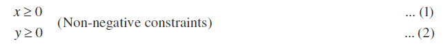
Let x be the number of tables and y be the number of chairs that the dealer buys. Obviously, x and y must be non-negative, i.e.,
The dealer is constrained by the maximum amount he can invest (Here it is
Rs 50,000) and by the maximum number of items he can store (Here it is 60).
Stated mathematically,
2500x + 500y ≤ 50000 (investment constraint)
or 5x + y ≤ 100 ... (3)
and x + y ≤ 60 (storage constraint) ... (4)
The dealer wants to invest in such a way so as to maximise his profit, say, Z which stated as a function of x and y is given by
Z = 250x + 75y (called objective function) ... (5)
Mathematically, the given problems now reduces to:
Maximise Z = 250x + 75y
subject to the constraints:
5x + y ≤ 100
x + y ≤ 60
x ≥ 0, y ≥ 0
So, we have to maximise the linear function Z subject to certain conditions determined by a set of linear inequalities with variables as non-negative. There are also some other problems where we have to minimise a linear function subject to certain conditions determined by a set of linear inequalities with variables as non-negative. Such problems are called Linear Programming Problems.
Thus, a Linear Programming Problem is one that is concerned with finding the optimal value (maximum or minimum value) of a linear function (called objective function) of several variables (say x and y), subject to the conditions that the variables are non-negative and satisfy a set of linear inequalities (called linear constraints). The term linear implies that all the mathematical relations used in the problem are linear relations while the term programming refers to the method of determining a particular programme or plan of action.
Before we proceed further, we now formally define some terms (which have been used above) which we shall be using in the linear programming problems:
Objective function Linear function Z = ax + by, where a, b are constants, which has to be maximised or minimized is called a linear objective function.
In the above example, Z = 250x + 75y is a linear objective function. Variables x and y are called decision variables.
Constraints The linear inequalities or equations or restrictions on the variables of a linear programming problem are called constraints. The conditions x ≥ 0, y ≥ 0 are called non-negative restrictions. In the above example, the set of inequalities (1) to (4) are constraints.
Optimisation problem A problem which seeks to maximise or minimise a linear function (say of two variables x and y) subject to certain constraints as determined by a set of linear inequalities is called an optimisation problem. Linear programming problems are special type of optimisation problems. The above problem of investing a given sum by the dealer in purchasing chairs and tables is an example of an optimisation problem as well as of a linear programming problem.
We will now discuss how to find solutions to a linear programming problem. In this chapter, we will be concerned only with the graphical method.
12.2.2 Graphical method of solving linear programming problems
In Class XI, we have learnt how to graph a system of linear inequalities involving two variables x and y and to find its solutions graphically. Let us refer to the problem of investment in tables and chairs discussed in Section 12.2. We will now solve this problem graphically. Let us graph the constraints stated as linear inequalities:
5x + y ≤ 100 ... (1)
x + y ≤ 60 ... (2)
x ≥ 0 ... (3)
y ≥ 0 ... (4)
The graph of this system (shaded region) consists of the points common to all half planes determined by the inequalities (1) to (4) (Fig 12.1). Each point in this region represents a feasible choice open to the dealer for investing in tables and chairs. The region, therefore, is called the feasible region for the problem. Every point of this region is called a feasible solution to the problem. Thus, we have,
Feasible region The common region determined by all the constraints including
non-negative constraints x, y ≥ 0 of a linear programming problem is called the feasible region (or solution region) for the problem. In Fig 12.1, the region OABC (shaded) is the feasible region for the problem. The region other than feasible region is called an infeasible region.
Feasible solutions Points within and on the boundary of the feasible region represent feasible solutions of the constraints. In Fig 12.1, every point within and on the boundary of the feasible region OABC represents feasible solution to the problem. For example, the point (10, 50) is a feasible solution of the problem and so are the points (0, 60), (20, 0) etc.
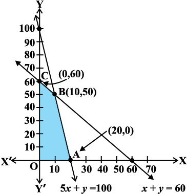
Fig 12.1
Any point outside the feasible region is called an infeasible solution. For example, the point (25, 40) is an infeasible solution of the problem.
Optimal (feasible) solution: Any point in the feasible region that gives the optimal value (maximum or minimum) of the objective function is called an optimal solution.
Now, we see that every point in the feasible region OABC satisfies all the constraints as given in (1) to (4), and since there are infinitely many points, it is not evident how we should go about finding a point that gives a maximum value of the objective function
Z = 250x + 75y. To handle this situation, we use the following theorems which are fundamental in solving linear programming problems. The proofs of these theorems are beyond the scope of the book.
Theorem 1 Let R be the feasible region (convex polygon) for a linear programming problem and let Z = ax + by be the objective function. When Z has an optimal value (maximum or minimum), where the variables x and y are subject to constraints described by linear inequalities, this optimal value must occur at a corner point* (vertex) of the feasible region.
Theorem 2 Let R be the feasible region for a linear programming problem, and let
Z = ax + by be the objective function. If R is bounded**, then the objective function Z has both a maximum and a minimum value on R and each of these occurs at a corner point (vertex) of R.
Remark If R is unbounded, then a maximum or a minimum value of the objective function may not exist. However, if it exists, it must occur at a corner point of R.
(By Theorem 1).
In the above example, the corner points (vertices) of the bounded (feasible) region are: O, A, B and C and it is easy to find their coordinates as (0, 0), (20, 0), (10, 50) and (0, 60) respectively. Let us now compute the values of Z at these points.
We have
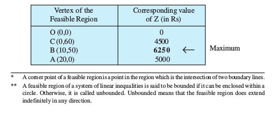
We observe that the maximum profit to the dealer results from the investment strategy (10, 50), i.e. buying 10 tables and 50 chairs.
This method of solving linear programming problem is referred as Corner Point Method. The method comprises of the following steps:
1. Find the feasible region of the linear programming problem and determine its corner points (vertices) either by inspection or by solving the two equations of the lines intersecting at that point.
3. (i) When the feasible region is bounded, M and m are the maximum and minimum values of Z.
(ii) In case, the feasible region is unbounded, we have:
4. (a) M is the maximum value of Z, if the open half plane determined by
ax + by > M has no point in common with the feasible region. Otherwise, Z has no maximum value.
(b) Similarly, m is the minimum value of Z, if the open half plane determined by
ax + by < m has no point in common with the feasible region. Otherwise, Z has no minimum value.
We will now illustrate these steps of Corner Point Method by considering some examples:
Example 1 Solve the following linear programming problem graphically:
Maximise Z = 4x + y ... (1)
subject to the constraints:
x + y ≤ 50 ... (2)
3x + y ≤ 90 ... (3)
x ≥ 0, y ≥ 0 ... (4)
Solution The shaded region in Fig 12.2 is the feasible region determined by the system of constraints (2) to (4). We observe that the feasible region OABC is bounded. So, we now use Corner Point Method to determine the maximum value of Z.
The coordinates of the corner points O, A, B and C are (0, 0), (30, 0), (20, 30) and (0, 50) respectively. Now we evaluate Z at each corner point.
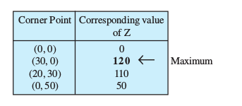
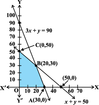
Fig 12.2
Hence, maximum value of Z is 120 at the point (30, 0).
Example 2 Solve the following linear programming problem graphically:
Minimise Z = 200 x + 500 y ... (1)
subject to the constraints:
x + 2y ≥ 10 ... (2)
3x + 4y ≤ 24 ... (3)
x ≥ 0, y ≥ 0 ... (4)
Solution The shaded region in Fig 12.3 is the feasible region ABC determined by the system of constraints (2) to (4), which is bounded. The coordinates of corner points A, B and C are (0,5), (4,3) and (0,6) respectively. Now we evaluate Z = 200x + 500y at these points.
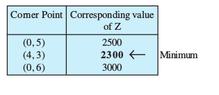
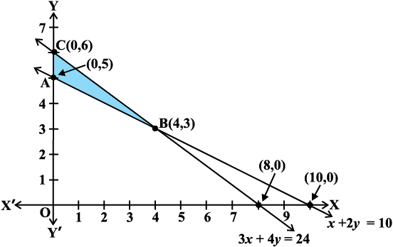
Fig 12.3
Example 3 Solve the following problem graphically:
Minimise and Maximise Z = 3x + 9y ... (1)
subject to the constraints: x + 3y ≤ 60 ... (2)
x + y ≥ 10 ... (3)
x ≤ y ... (4)
x ≥ 0, y ≥ 0 ... (5)
Solution First of all, let us graph the feasible region of the system of linear inequalities (2) to (5). The feasible region ABCD is shown in the Fig 12.4. Note that the region is bounded. The coordinates of the corner points A, B, C and D are (0, 10), (5, 5), (15,15) and (0, 20) respectively.
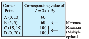
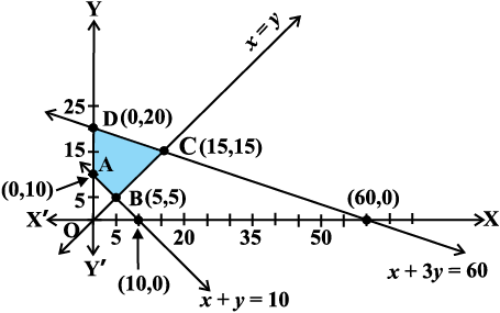
Fig 12.4
We now find the minimum and maximum value of Z. From the table, we find that the minimum value of Z is 60 at the point B (5, 5) of the feasible region.
The maximum value of Z on the feasible region occurs at the two corner points
C (15, 15) and D (0, 20) and it is 180 in each case.
Remark Observe that in the above example, the problem has multiple optimal solutions at the corner points C and D, i.e. the both points produce same maximum value 180. In such cases, you can see that every point on the line segment CD joining the two corner points C and D also give the same maximum value. Same is also true in the case if the two points produce same minimum value.
Example 4 Determine graphically the minimum value of the objective function
Z = – 50x + 20y ... (1)
subject to the constraints:
2x – y ≥ – 5 ... (2)
3x + y ≥ 3 ... (3)
2x – 3y ≤ 12 ... (4)
x ≥ 0, y ≥ 0 ... (5)
Solution First of all, let us graph the feasible region of the system of inequalities (2) to (5). The feasible region (shaded) is shown in the Fig 12.5. Observe that the feasible region is unbounded.
We now evaluate Z at the corner points.
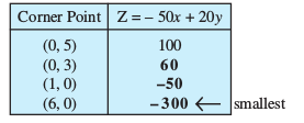
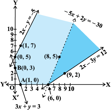
Fig 12.5
From this table, we find that – 300 is the smallest value of Z at the corner point
(6, 0). Can we say that minimum value of Z is – 300? Note that if the region would have been bounded, this smallest value of Z is the minimum value of Z (Theorem 2). But here we see that the feasible region is unbounded. Therefore, – 300 may or may not be the minimum value of Z. To decide this issue, we graph the inequality
– 50x + 20y < – 300 (see Step 3(ii) of corner Point Method.)
i.e., – 5x + 2y < – 30
and check whether the resulting open half plane has points in common with feasible region or not. If it has common points, then –300 will not be the minimum value of z. Otherwise, –300 will be the minimum value of Z.
As shown in the Fig 12.5, it has common points. Therefore, Z = –50 x + 20 y
has no minimum value subject to the given constraints.
In the above example, can you say whether z = – 50 x + 20 y has the maximum value 100 at (0,5)? For this, check whether the graph of – 50 x + 20 y > 100 has points in common with the feasible region. (Why?)
Example 5 Minimise Z = 3x + 2y
subject to the constraints:
x + y ≥ 8 ... (1)
3x + 5y ≤ 15 ... (2)
x ≥ 0, y ≥ 0 ... (3)
Solution Let us graph the inequalities (1) to (3) (Fig 12.6). Is there any feasible region? Why is so?
From Fig 12.6, you can see that there is no point satisfying all the constraints simultaneously. Thus, the problem is having no feasible region and hence no feasible solution.
Fig 12.6
Remarks From the examples which we have discussed so far, we notice some general features of linear programming problems:
(i) The feasible region is always a convex region.
(ii) The maximum (or minimum) solution of the objective function occurs at the vertex (corner) of the feasible region. If two corner points produce the same maximum (or minimum) value of the objective function, then every point on the line segment joining these points will also give the same maximum (or minimum) value.
EXERCISE 12.1
Solve the following Linear Programming Problems graphically:
1. Maximise Z = 3x + 4y
subject to the constraints : x + y ≤ 4, x ≥ 0, y ≥ 0.
2. Minimise Z = – 3x + 4 y
subject to x + 2y ≤ 8, 3x + 2y ≤ 12, x ≥ 0, y ≥ 0.
3. Maximise Z = 5x + 3y
subject to 3x + 5y ≤ 15, 5x + 2y ≤ 10, x ≥ 0, y ≥ 0.
4. Minimise Z = 3x + 5y
such that x + 3y ≥ 3, x + y ≥ 2, x, y ≥ 0.
5. Maximise Z = 3x + 2y
subject to x + 2y ≤ 10, 3x + y ≤ 15, x, y ≥ 0.
6. Minimise Z = x + 2y
subject to 2x + y ≥ 3, x + 2y ≥ 6, x, y ≥ 0.
Show that the minimum of Z occurs at more than two points.
7. Minimise and Maximise Z = 5x + 10 y
subject to x + 2y ≤ 120, x + y ≥ 60, x – 2y ≥ 0, x, y ≥ 0.
8. Minimise and maximise Z = x + 2y
subject to x + 2y ≥ 100, 2x – y ≤ 0, 2x + y ≤ 200; x, y ≥ 0.
9. Maximise Z = – x + 2y, subject to the constraints:
x ≥ 3, x + y ≥ 5, x + 2y ≥ 6, y ≥ 0.
10. Maximise Z = x + y, subject to x – y ≤ –1, –x + y ≤ 0, x, y ≥ 0.
12.3 Different Types of Linear Programming Problems
A few important linear programming problems are listed below:
1. Manufacturing problems In these problems, we determine the number of units of different products which should be produced and sold by a firm
when each product requires a fixed manpower, machine hours, labour hour per unit of product, warehouse space per unit of the output etc., in order to make maximum profit.
2. Diet problems In these problems, we determine the amount of different kinds of constituents/nutrients which should be included in a diet so as to minimise the cost of the desired diet such that it contains a certain minimum amount of each constituent/nutrients.
3. Transportation problems In these problems, we determine a transportation schedule in order to find the cheapest way of transporting a product from
plants/factories situated at different locations to different markets.
Let us now solve some of these types of linear programming problems:
Example 6 (Diet problem): A dietician wishes to mix two types of foods in such a way that vitamin contents of the mixture contain atleast 8 units of vitamin A and 10 units of vitamin C. Food ‘I’ contains 2 units/kg of vitamin A and 1 unit/kg of vitamin C. Food ‘II’ contains 1 unit/kg of vitamin A and 2 units/kg of vitamin C. It costs
Rs 50 per kg to purchase Food ‘I’ and Rs 70 per kg to purchase Food ‘II’. Formulate this problem as a linear programming problem to minimise the cost of such a mixture.
Solution Let the mixture contain x kg of Food ‘I’ and y kg of Food ‘II’. Clearly, x ≥ 0, y ≥ 0. We make the following table from the given data:
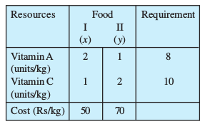
Since the mixture must contain at least 8 units of vitamin A and 10 units of
vitamin C, we have the constraints:
x + 2y ≥ 10
Total cost Z of purchasing x kg of food ‘I’ and y kg of Food ‘II’ is
Z = 50x + 70y
Hence, the mathematical formulation of the problem is:
Minimise Z = 50x + 70y ... (1)
subject to the constraints:
2x + y ≥ 8 ... (2)
x + 2y ≥ 10 ... (3)
x, y ≥ 0 ... (4)
Let us graph the inequalities (2) to (4). The feasible region determined by the system is shown in the Fig 12.7. Here again, observe that the feasible region is unbounded.
Let us evaluate Z at the corner points A(0,8), B(2,4) and C(10,0).
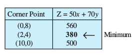
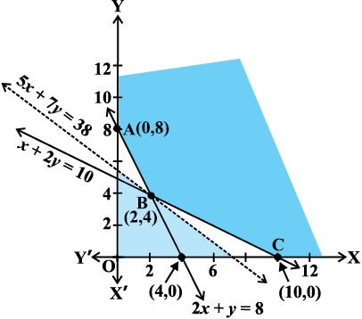
50x + 70y < 380 i.e., 5x + 7y < 38
to check whether the resulting open half plane has any point common with the feasible region. From the Fig 12.7, we see that it has no points in common.
Thus, the minimum value of Z is 380 attained at the point (2, 4). Hence, the optimal mixing strategy for the dietician would be to mix 2 kg of Food ‘I’ and 4 kg of Food ‘II’, and with this strategy, the minimum cost of the mixture will be Rs 380.
Example 7 (Allocation problem) A cooperative society of farmers has 50 hectare of land to grow two crops X and Y. The profit from crops X and Y per hectare are estimated as Rs 10,500 and Rs 9,000 respectively. To control weeds, a liquid herbicide has to be used for crops X and Y at rates of 20 litres and 10 litres per hectare. Further, no more than 800 litres of herbicide should be used in order to protect fish and wild life using a pond which collects drainage from this land. How much land should be allocated to each crop so as to maximise the total profit of the society?
Solution Let x hectare of land be allocated to crop X and y hectare to crop Y. Obviously, x ≥ 0, y ≥ 0.
Profit per hectare on crop X = Rs 10500
Profit per hectare on crop Y = Rs 9000
Therefore, total profit = Rs (10500x + 9000y)
The mathematical formulation of the problem is as follows:
Maximise Z = 10500 x + 9000 y
subject to the constraints:
x + y ≤ 50 (constraint related to land) ... (1)
20x + 10y ≤ 800 (constraint related to use of herbicide)
i.e. 2x + y ≤ 80 ... (2)
x ≥ 0, y ≥ 0 (non negative constraint) ... (3)
Let us draw the graph of the system of inequalities (1) to (3). The feasible region OABC is shown (shaded) in the Fig 12.8. Observe that the feasible region is bounded.
The coordinates of the corner points O, A, B and C are (0, 0), (40, 0), (30, 20) and (0, 50) respectively. Let us evaluate the objective function Z = 10500 x + 9000y at these vertices to find which one gives the maximum profit.
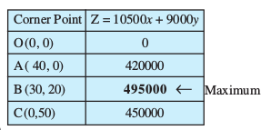
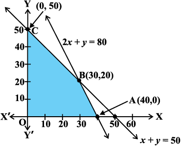
Fig 12.8
Hence, the society will get the maximum profit of Rs 4,95,000 by allocating 30 hectares for crop X and 20 hectares for crop Y.
Example 8 (Manufacturing problem) A manufacturing company makes two models A and B of a product. Each piece of Model A requires 9 labour hours for fabricating and 1 labour hour for finishing. Each piece of Model B requires 12 labour hours for fabricating and 3 labour hours for finishing. For fabricating and finishing, the maximum labour hours available are 180 and 30 respectively. The company makes a profit of Rs 8000 on each piece of model A and Rs 12000 on each piece of Model B. How many pieces of Model A and Model B should be manufactured per week to realise a maximum profit? What is the maximum profit per week?
Total profit (in Rs) = 8000 x + 12000 y
Let Z = 8000 x + 12000 y
We now have the following mathematical model for the given problem.
Maximise Z = 8000 x + 12000 y ... (1)
subject to the constraints:
9x + 12y ≤ 180 (Fabricating constraint)
i.e. 3x + 4y ≤ 60 ... (2)
x + 3y ≤ 30 (Finishing constraint) ... (3)
x ≥ 0, y ≥ 0 (non-negative constraint) ... (4)
The feasible region (shaded) OABC determined by the linear inequalities (2) to (4) is shown in the Fig 12.9. Note that the feasible region is bounded.
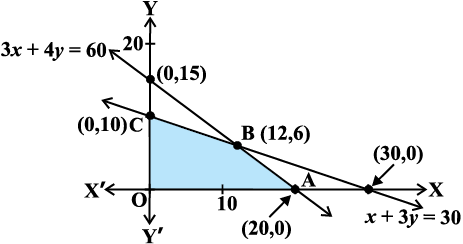
Fig 12.9
Let us evaluate the objective function Z at each corner point as shown below:
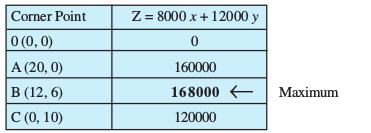
We find that maximum value of Z is 1,68,000 at B (12, 6). Hence, the company should produce 12 pieces of Model A and 6 pieces of Model B to realise maximum profit and maximum profit then will be Rs 1,68,000.
EXERCISE 12.2
1. Reshma wishes to mix two types of food P and Q in such a way that the vitamin contents of the mixture contain at least 8 units of vitamin A and 11 units of vitamin B. Food P costs Rs 60/kg and Food Q costs Rs 80/kg. Food P contains 3 units/kg of Vitamin A and 5 units / kg of Vitamin B while food Q contains 4 units/kg of Vitamin A and 2 units/kg of vitamin B. Determine the minimum cost of the mixture.
2. One kind of cake requires 200g of flour and 25g of fat, and another kind of cake requires 100g of flour and 50g of fat. Find the maximum number of cakes which can be made from 5kg of flour and 1 kg of fat assuming that there is no shortage of the other ingredients used in making the cakes.
3. A factory makes tennis rackets and cricket bats. A tennis racket takes 1.5 hours of machine time and 3 hours of craftman’s time in its making while a cricket bat takes 3 hour of machine time and 1 hour of craftman’s time. In a day, the factory has the availability of not more than 42 hours of machine time and 24 hours of craftsman’s time.
(i) What number of rackets and bats must be made if the factory is to work at full capacity?
(ii) If the profit on a racket and on a bat is Rs 20 and Rs 10 respectively, find the maximum profit of the factory when it works at full capacity.
4. A manufacturer produces nuts and bolts. It takes 1 hour of work on machine A and 3 hours on machine B to produce a package of nuts. It takes 3 hours on machine A and 1 hour on machine B to produce a package of bolts. He earns a profit of Rs17.50 per package on nuts and Rs 7.00 per package on bolts. How many packages of each should be produced each day so as to maximise his profit, if he operates his machines for at the most 12 hours a day?
5. A factory manufactures two types of screws, A and B. Each type of screw requires the use of two machines, an automatic and a hand operated. It takes 4 minutes on the automatic and 6 minutes on hand operated machines to manufacture a package of screws A, while it takes 6 minutes on automatic and 3 minutes on the hand operated machines to manufacture a package of screws B. Each machine is available for at the most 4 hours on any day. The manufacturer can sell a package of screws A at a profit of Rs 7 and screws B at a profit of
Rs 10. Assuming that he can sell all the screws he manufactures, how many packages of each type should the factory owner produce in a day in order to maximise his profit? Determine the maximum profit.
6. A cottage industry manufactures pedestal lamps and wooden shades, each requiring the use of a grinding/cutting machine and a sprayer. It takes 2 hours on grinding/cutting machine and 3 hours on the sprayer to manufacture a pedestal lamp. It takes 1 hour on the grinding/cutting machine and 2 hours on the sprayer to manufacture a shade. On any day, the sprayer is available for at the most 20 hours and the grinding/cutting machine for at the most 12 hours. The profit from the sale of a lamp is Rs 5 and that from a shade is Rs 3. Assuming that the manufacturer can sell all the lamps and shades that he produces, how should he schedule his daily production in order to maximise his profit?
7. A company manufactures two types of novelty souvenirs made of plywood. Souvenirs of type A require 5 minutes each for cutting and 10 minutes each for assembling. Souvenirs of type B require 8 minutes each for cutting and 8 minutes each for assembling. There are 3 hours 20 minutes available for cutting and 4 hours for assembling. The profit is Rs 5 each for type A and Rs 6 each for type B souvenirs. How many souvenirs of each type should the company manufacture in order to maximise the profit?
8. A merchant plans to sell two types of personal computers – a desktop model and a portable model that will cost Rs 25000 and Rs 40000 respectively. He estimates that the total monthly demand of computers will not exceed 250 units. Determine the number of units of each type of computers which the merchant should stock to get maximum profit if he does not want to invest more than Rs 70 lakhs and if his profit on the desktop model is Rs 4500 and on portable model is Rs 5000.
9. A diet is to contain at least 80 units of vitamin A and 100 units of minerals. Two foods F1 and F2 are available. Food F1 costs Rs 4 per unit food and F2 costs
Rs 6 per unit. One unit of food F1 contains 3 units of vitamin A and 4 units of minerals. One unit of food F2 contains 6 units of vitamin A and 3 units of minerals. Formulate this as a linear programming problem. Find the minimum cost for diet that consists of mixture of these two foods and also meets the minimal nutritional requirements.
10. There are two types of fertilisers F1 and F2. F1 consists of 10% nitrogen and 6% phosphoric acid and F2 consists of 5% nitrogen and 10% phosphoric acid. After testing the soil conditions, a farmer finds that she needs atleast 14 kg of nitrogen and 14 kg of phosphoric acid for her crop. If F1 costs Rs 6/kg and F2 costs
Rs 5/kg, determine how much of each type of fertiliser should be used so that nutrient requirements are met at a minimum cost. What is the minimum cost?
11. The corner points of the feasible region determined by the following system of linear inequalities:
2x + y ≤ 10, x + 3y ≤ 15, x, y ≥ 0 are (0, 0), (5, 0), (3, 4) and (0, 5). Let Z = px + qy, where p, q > 0. Condition on p and q so that the maximum of Z occurs at both (3, 4) and (0, 5) is
(A) p = q (B) p = 2q (C) p = 3q (D) q = 3p
Miscellaneous Examples
Example 9 (Diet problem) A dietician has to develop a special diet using two foods P and Q. Each packet (containing 30 g) of food P contains 12 units of calcium, 4 units of iron, 6 units of cholesterol and 6 units of vitamin A. Each packet of the same quantity of food Q contains 3 units of calcium, 20 units of iron, 4 units of cholesterol and 3 units of vitamin A. The diet requires atleast 240 units of calcium, atleast 460 units of iron and at most 300 units of cholesterol. How many packets of each food should be used to minimise the amount of vitamin A in the diet? What is the minimum amount of vitamin A?
Solution Let x and y be the number of packets of food P and Q respectively. Obviously x ≥ 0, y ≥ 0. Mathematical formulation of the given problem is as follows:
Minimise z = 6x + 3y (vitamin A)
subject to the constraints
12x + 3y ≥ 240 (constraint on calcium), i.e. 4x + y ≥ 80 ... (1)
4x + 20y ≥ 460 (constraint on iron), i.e. x + 5y ≥ 115 ... (2)
6x + 4y ≤ 300 (constraint on cholesterol), i.e. 3x + 2y ≤ 150 ... (3)
x ≥ 0, y ≥ 0 ... (4)
Let us graph the inequalities (1) to (4).
The feasible region (shaded) determined by the constraints (1) to (4) is shown in
Fig 12.10 and note that it is bounded.
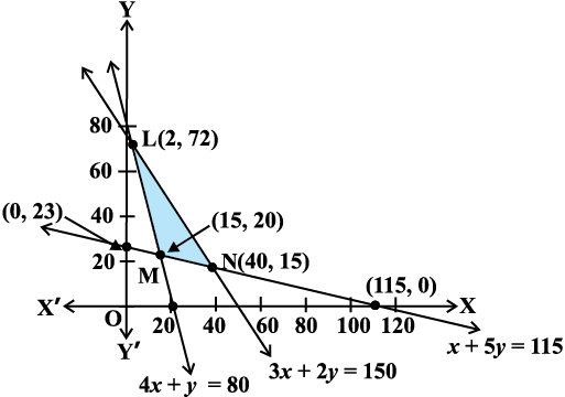
Fig 12.10
The coordinates of the corner points L, M and N are (2, 72), (15, 20) and (40, 15) respectively. Let us evaluate Z at these points:
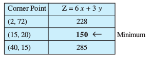
From the table, we find that Z is minimum at the point (15, 20). Hence, the amount of vitamin A under the constraints given in the problem will be minimum, if 15 packets of food P and 20 packets of food Q are used in the special diet. The minimum amount of vitamin A will be 150 units.
Example 10 (Manufacturing problem) A manufacturer has three machines I, II and III installed in his factory. Machines I and II are capable of being operated for
at most 12 hours whereas machine III must be operated for atleast 5 hours a day. She produces only two items M and N each requiring the use of all the three machines.
The number of hours required for producing 1 unit of each of M and N on the three machines are given in the following table:
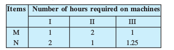
She makes a profit of Rs 600 and Rs 400 on items M and N respectively. How many of each item should she produce so as to maximise her profit assuming that she can sell all the items that she produced? What will be the maximum profit?
Solution Let x and y be the number of items M and N respectively.
Total profit on the production = Rs (600 x + 400 y)
Mathematical formulation of the given problem is as follows:
Maximise Z = 600 x + 400 y
subject to the constraints:
x + 2y ≤ 12 (constraint on Machine I) ... (1)
2x + y ≤ 12 (constraint on Machine II) ... (2)
x + ![]() y ≥ 5 (constraint on Machine III) ... (3)
y ≥ 5 (constraint on Machine III) ... (3)
x ≥ 0, y ≥ 0 ... (4)
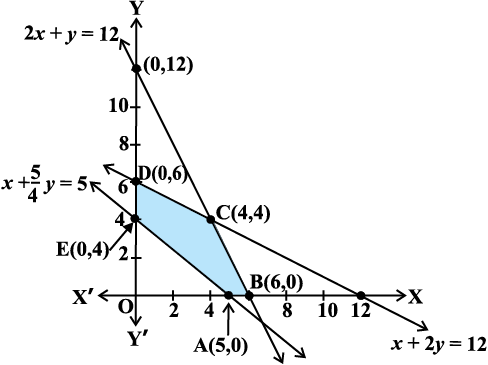
Let us draw the graph of constraints (1) to (4). ABCDE is the feasible region (shaded) as shown in Fig 12.11 determined by the constraints (1) to (4). Observe that the feasible region is bounded, coordinates of the corner points A, B, C, D and E are
(5, 0) (6, 0), (4, 4), (0, 6) and (0, 4) respectively.
Let us evaluate Z = 600 x + 400 y at these corner points.
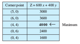
We see that the point (4, 4) is giving the maximum value of Z. Hence, the manufacturer has to produce 4 units of each item to get the maximum profit of Rs 4000.
Example 11 (Transportation problem) there are two factories located one at place P and the other at place Q. From these locations, a certain commodity is to be delivered to each of the three depots situated at A, B and C. The weekly requirements of the depots are respectively 5, 5 and 4 units of the commodity while the production capacity of the factories at P and Q are respectively 8 and 6 units. The cost of transportation per unit is given below:
How many units should be transported from each factory to each depot in order that the transportation cost is minimum. What will be the minimum transportation cost?
Solution The problem can be explained diagrammatically as follows (Fig 12.12):
Let x units and y units of the commodity be transported from the factory at P to
the depots at A and B respectively. Then (8 – x – y) units will be transported to depot
at C (Why?)
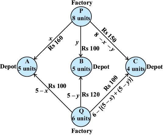
Fig 12.12
Hence, we have x ≥ 0, y ≥ 0 and 8 – x – y ≥ 0
i.e. x ≥ 0, y ≥ 0 and x + y ≤ 8
Now, the weekly requirement of the depot at A is 5 units of the commodity. Since x units are transported from the factory at P, the remaining (5 – x) units need to be transported from the factory at Q. Obviously, 5 – x ≥ 0, i.e. x ≤ 5.
Similarly, (5 – y) and 6 – (5 – x + 5 – y) = x + y – 4 units are to be transported from the factory at Q to the depots at B and C respectively.
Thus, 5 – y ≥ 0 , x + y – 4 ≥ 0
i.e. y ≤ 5 , x + y ≥ 4
Total transportation cost Z is given by
Z = 160 x + 100 y + 150 (8 – x – y) + 100 ( 5 – x) + 120 (5 – y) + 100 (x + y – 4)
= 10 (x – 7 y + 190)
Therefore, the problem reduces to
Minimise Z = 10 (x – 7y + 190)
subject to the constraints:
x ≥ 0, y ≥ 0 ... (1)
x + y ≤ 8 ... (2)
x ≤ 5 ... (3)
y ≤ 5 ... (4)
and x + y ≥ 4 ... (5)
The shaded region ABCDEF represented by the constraints (1) to (5) is the feasible region (Fig 12.13).
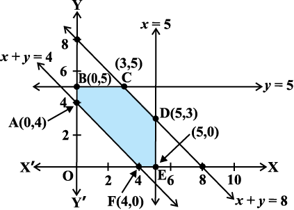
Fig 12.13
Observe that the feasible region is bounded. The coordinates of the corner points of the feasible region are (0, 4), (0, 5), (3, 5), (5, 3), (5, 0) and (4, 0).
Let us evaluate Z at these points.
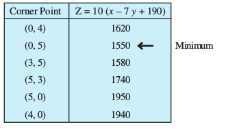
From the table, we see that the minimum value of Z is 1550 at the point (0, 5).
Hence, the optimal transportation strategy will be to deliver 0, 5 and 3 units from the factory at P and 5, 0 and 1 units from the factory at Q to the depots at A, B and C respectively. Corresponding to this strategy, the transportation cost would be minimum, i.e., Rs 1550.
Miscellaneous Exercise on Chapter 12
1. Refer to Example 9. How many packets of each food should be used to maximise the amount of vitamin A in the diet? What is the maximum amount of vitamin A in the diet?
2. A farmer mixes two brands P and Q of cattle feed. Brand P, costing Rs 250 per bag, contains 3 units of nutritional element A, 2.5 units of element B and 2 units of element C. Brand Q costing Rs 200 per bag contains 1.5 units of nutritional element A, 11.25 units of element B, and 3 units of element C. The minimum requirements of nutrients A, B and C are 18 units, 45 units and 24 units respectively. Determine the number of bags of each brand which should be mixed in order to produce a mixture having a minimum cost per bag? What is the minimum cost of the mixture per bag?
3. A dietician wishes to mix together two kinds of food X and Y in such a way that the mixture contains at least 10 units of vitamin A, 12 units of vitamin B and 8 units of vitamin C. The vitamin contents of one kg food is given below:
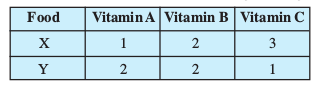
One kg of food X costs Rs 16 and one kg of food Y costs Rs 20. Find the least cost of the mixture which will produce the required diet?
4. A manufacturer makes two types of toys A and B. Three machines are needed for this purpose and the time (in minutes) required for each toy on the machines is given below:
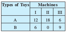
Each machine is available for a maximum of 6 hours per day. If the profit on each toy of type A is Rs 7.50 and that on each toy of type B is Rs 5, show that 15 toys of type A and 30 of type B should be manufactured in a day to get maximum profit.
5. An aeroplane can carry a maximum of 200 passengers. A profit of Rs 1000 is made on each executive class ticket and a profit of Rs 600 is made on each economy class ticket. The airline reserves at least 20 seats for executive class. However, at least 4 times as many passengers prefer to travel by economy class than by the executive class. Determine how many tickets of each type must be sold in order to maximise the profit for the airline. What is the maximum profit?
6. Two godowns A and B have grain capacity of 100 quintals and 50 quintals respectively. They supply to 3 ration shops, D, E and F whose requirements are 60, 50 and 40 quintals respectively. The cost of transportation per quintal from the godowns to the shops are given in the following table:
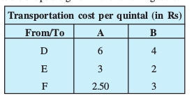
How should the supplies be transported in order that the transportation cost is minimum? What is the minimum cost?
7. An oil company has two depots A and B with capacities of 7000 L and 4000 L respectively. The company is to supply oil to three petrol pumps, D, E and F whose requirements are 4500L, 3000L and 3500L respectively. The distances (in km) between the depots and the petrol pumps is given in the following table:
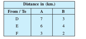
Assuming that the transportation cost of 10 litres of oil is Re 1 per km, how should the delivery be scheduled in order that the transportation cost is minimum? What is the minimum cost?
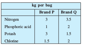
8. A fruit grower can use two types of fertilizer in his garden, brand P and brand Q. The amounts (in kg) of nitrogen, phosphoric acid, potash, and chlorine in a bag of each brand are given in the table. Tests indicate that the garden needs at least 240 kg of phosphoric acid, at least 270 kg of potash and at most 310 kg of chlorine.
If the grower wants to minimise the amount of nitrogen added to the garden, how many bags of each brand should be used? What is the minimum amount of nitrogen added in the garden?
9. Refer to Question 8. If the grower wants to maximise the amount of nitrogen added to the garden, how many bags of each brand should be added? What is the maximum amount of nitrogen added?
10. A toy company manufactures two types of dolls, A and B. Market research and available resources have indicated that the combined production level should not exceed 1200 dolls per week and the demand for dolls of type B is at most half of that for dolls of type A. Further, the production level of dolls of type A can exceed three times the production of dolls of other type by at most 600 units. If the company makes profit of Rs 12 and Rs 16 per doll respectively on dolls A and B, how many of each should be produced weekly in order to maximise the profit?
Summary
- A linear programming problem is one that is concerned with finding the optimal value (maximum or minimum) of a linear function of several variables (called objective function) subject to the conditions that the variables are
- A few important linear programming problems are:
(i) Diet problems
(ii) Manufacturing problems
(iii) Transportation problems
- The common region determined by all the constraints including the non-negative constraints x ≥ 0, y ≥ 0 of a linear programming problem is called the feasible region (or solution region) for the problem.
- Points within and on the boundary of the feasible region represent feasible solutions of the constraints.
Any point outside the feasible region is an infeasible solution.
- Any point in the feasible region that gives the optimal value (maximum or minimum) of the objective function is called an optimal solution.
- The following Theorems are fundamental in solving linear programming problems:
Theorem 1 Let R be the feasible region (convex polygon) for a linear programming problem and let Z = ax + by be the objective function. When Z has an optimal value (maximum or minimum), where the variables x and y are subject to constraints described by linear inequalities, this optimal value must occur at a corner point (vertex) of the feasible region.
Theorem 2 Let R be the feasible region for a linear programming problem, and let Z = ax + by be the objective function. If R is bounded, then the objective function Z has both a maximum and a minimum value on R and each of these occurs at a corner point (vertex) of R.
- If the feasible region is unbounded, then a maximum or a minimum may not exist. However, if it exists, it must occur at a corner point of R.
- Corner point method for solving a linear programming problem. The method comprises of the following steps:
(i) Find the feasible region of the linear programming problem and determine its corner points (vertices).
(ii) Evaluate the objective function Z = ax + by at each corner point. Let M and m respectively be the largest and smallest values at these points.
(iii) If the feasible region is bounded, M and m respectively are the maximum and minimum values of the objective function.
If the feasible region is unbounded, then
(i) M is the maximum value of the objective function, if the open half plane determined by ax + by >M has no point in common with the feasible region. Otherwise, the objective function has no maximum value.
(ii) m is the minimum value of the objective function, if the open half plane determined by ax + by <m has no point in common with the feasible region. Otherwise, the objective function has no minimum value.
- If two corner points of the feasible region are both optimal solutions of the same type, i.e., both produce the same maximum or minimum, then any point on the line segment joining these two points is also an optimal solution of the same type.
Historical Note
In the World War II, when the war operations had to be planned to economise expenditure, maximise damage to the enemy, linear programming problems came to the forefront.
The first problem in linear programming was formulated in 1941 by the Russian mathematician, L. Kantorovich and the American economist, F. L. Hitchcock, both of whom worked at it independently of each other. This was the well known transportation problem. In 1945, an English economist, G.Stigler, described yet another linear programming problem – that of determining an optimal diet.
In 1947, the American economist, G. B. Dantzig suggested an efficient method known as the simplex method which is an iterative procedure to solve any linear programming problem in a finite number of steps.
L. Katorovich and American mathematical economist, T. C. Koopmans were awarded the nobel prize in the year 1975 in economics for their pioneering work in linear programming. With the advent of computers and the necessary softwares, it has become possible to apply linear programming model to increasingly complex problems in many areas.