Table of Contents
Chapter Three
Motion in a Plane

3.1 Introduction
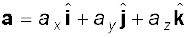
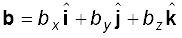
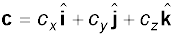
3.2 Scalars and vectors
3.3 Multiplication of vectors by real numbers
3.4 Addition and subtraction of vectors — graphical method
3.5 Resolution of vectors
3.6 Vector addition — analytical method
3.7 Motion in a plane
3.8 Motion in a plane with constant acceleration
3.9 Relative velocity in two dimensions
3.10 Projectile motion
3.11 Uniform circular motion
Summary
Points to ponder
Exercises
Additional exercises
3.1 Introduction
In the last chapter we developed the concepts of position, displacement, velocity and acceleration that are needed to describe the motion of an object along a straight line. We found that the directional aspect of these quantities can be taken care of by + and – signs, as in one dimension only two directions are possible. But in order to describe motion of an object in two dimensions (a plane) or three dimensions (space), we need to use vectors to describe the above-mentioned physical quantities. Therefore, it is first necessary to learn the language of vectors. What is a vector? How to add, subtract and multiply vectors ? What is the result of multiplying a vector by a real number ? We shall learn this to enable us to use vectors for defining velocity and acceleration in a plane. We then discuss motion of an object in a plane. As a simple case of motion in a plane, we shall discuss motion with constant acceleration and treat in detail the projectile motion. Circular motion is a familiar class of motion that has a special significance in daily-life situations. We shall discuss uniform circular motion in some detail.
The equations developed in this chapter for motion in a plane can be easily extended to the case of three dimensions.
3.2 Scalars and vectors
In physics, we can classify quantities as scalars or vectors. Basically, the difference is that a direction is associated with a vector but not with a scalar. A scalar quantity is a quantity with magnitude only. It is specified completely by a single number, along with the proper unit. Examples are : the distance between two points, mass of an object, the temperature of a body and the time at which a certain event happened. The rules for combining scalars are the rules of ordinary algebra. Scalars can be added, subtracted, multiplied and divided just as the ordinary numbers*. For example, if the length and breadth of a rectangle are 1.0 m and 0.5 m respectively, then its perimeter is the sum of the lengths of the four sides, 1.0 m + 0.5 m +1.0 m + 0.5 m = 3.0 m. The length of each side is a scalar and the perimeter is also a scalar. Take another example: the maximum and minimum temperatures on a particular day are 35.6 °C and 24.2 °C respectively. Then, the difference between the two temperatures is 11.4 °C. Similarly, if a uniform solid cube of aluminium of side 10 cm has a mass of 2.7 kg, then its volume is 10–3 m3 (a scalar) and its density is 2.7×10³ kg m–3 (a scalar).
A vector quantity is a quantity that has both a magnitude and a direction and obeys the triangle law of addition or equivalently the parallelogram law of addition. So, a vector is specified by giving its magnitude by a number and its direction. Some physical quantities that are represented by vectors are displacement, velocity, acceleration and force.
To represent a vector, we use a bold face type in this book. Thus, a velocity vector can be represented by a symbol v. Since bold face is difficult to produce, when written by hand, a vector is often represented by an arrow placed over a letter, say 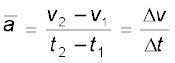 . Thus, both v and
  represent the velocity vector. The magnitude of a vector is often called its absolute value, indicated by |v| = v. Thus, a vector is represented by a bold face, e.g. by A, a, p, q, r, ... x, y, with respective magnitudes denoted by light face A, a, p, q, r, ... x, y.
3.2.1 Position and Displacement Vectors
To describe the position of an object moving in a plane, we need to choose a convenient point, say O as origin. Let P and P′ be the positions of the object at time t and t′, respectively [Fig.3.1(a)]. We join O and P by a straight line. Then, OP is the position vector of the object at time t. An arrow is marked at the head of this line. It is represented by a symbol r, i.e. OP = r. Point P′ is represented by another position vector, OP′ denoted by r′. The length of the vector r represents the magnitude of the vector and its direction is the direction in which P lies as seen from O. If the object moves from P to P′, the vector PP′ (with tail at P and tip at P′) is called the displacement vector corresponding to motion from point P (at time t) to point P′ (at time t′)
Fig. 3.1 (a) Position and displacement vectors. (b) Displacement vector PQ and different courses of motion.
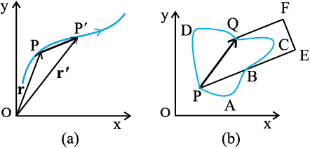
It is important to note that displacement vector is the straight line joining the initial and final positions and does not depend on the actual path undertaken by the object between the two positions. For example, in Fig. 4.1(b), given the initial and final positions as P and Q, the displacement vector is the same PQ for different paths of journey, say PABCQ, PDQ, and PBEFQ. Therefore, the magnitude of displacement is either less or equal to the path length of an object between two points. This fact was emphasised in the previous chapter also while discussing motion along a straight line.
* Addition and subtraction of scalars make sense only for quantities with same units. However, you can multiply and divide scalars of different units.
** In our study, vectors do not have fixed locations. So displacing a vector parallel to itself leaves the vector unchanged. Such vectors are called free vectors. However, in some physical applications, location or line of application of a vector is important. Such vectors are called localised vectors.
3.2.2 Equality of Vectors
Two vectors A and B are said to be equal if, and only if, they have the same magnitude and the same direction.**
Figure 3.2(a) shows two equal vectors A and B. We can easily check their equality. Shift B parallel to itself until its tail Q coincides with that of A, i.e. Q coincides with O. Then, since their tips S and P also coincide, the two vectors are said to be equal. In general, equality is indicated as A = B. Note that in Fig. 4.2(b), vectors A′ and B′ have the same magnitude but they are not equal because they have different directions. Even if we shift B′ parallel to itself so that its tail Q′ coincides with the tail O′ of A′, the tip S′ of B′ does not coincide with the tip P′ of A′.
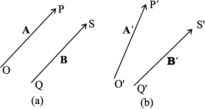
Fig. 3.2 (a) Two equal vectors A and B. (b) Two vectors A′ and B′ are unequal though they are of the same length.
3.3 Multiplication of vectors by real numbers
Multiplying a vector A with a positive number λ gives a vector whose magnitude is changed by the factor λ but the direction is the same as that of A :
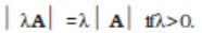
For example, if A is multiplied by 2, the resultant vector 2A is in the same direction as A and has a magnitude twice of |A| as shown in Fig. 3.3(a).
Multiplying a vector A by a negative number −λ gives another vector whose direction is opposite to the direction of A and whose magnitude is λ times |A|.
Multiplying a given vector A by negative numbers, say –1 and –1.5, gives vectors as shown in Fig 3.3(b).
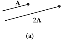
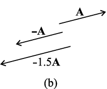
Fig. 3.3 (a) Vector A and the resultant vector after multiplying A by a positive number 2. (b) Vector A and resultant vectors after multiplying it by a negative number –1 and –1.5.
The factor λ by which a vector A is multiplied could be a scalar having its own physical dimension. Then, the dimension of λ A is the product of the dimensions of λ and A. For example, if we multiply a constant velocity vector by duration (of time), we get a displacement vector.
3.4 Addition and subtraction of vectors — graphical method
As mentioned in section 4.2, vectors, by definition, obey the triangle law or equivalently, the parallelogram law of addition. We shall now describe this law of addition using the graphical method. Let us consider two vectors A and B that lie in a plane as shown in Fig. 4.4(a).
Fig. 3.4 (a) Vectors A and B. (b) Vectors A and B added graphically. (c) Vectors B and A added graphically. (d) Illustrating the associative law of vector addition.
The lengths of the line segments representing these vectors are proportional to the magnitude of the vectors. To find the sum A + B, we place vector B so that its tail is at the head of the vector A, as in Fig. 3.4(b). Then, we join the tail of A to the head of B. This line OQ represents a vector R, that is, the sum of the vectors A and B. Since, in this procedure of vector addition, vectors are arranged head to tail, this graphical method is called the head-to-tail method. The two vectors and their resultant form three sides of a triangle, so this method is also known as triangle method of vector addition. If we find the resultant of
B + A as in Fig. 3.4(c), the same vector R is obtained. Thus, vector addition is commutative:
A + B = B + A (3.1)
The addition of vectors also obeys the associative law as illustrated in Fig. 3.4(d). The result of adding vectors A and B first and then adding vector C is the same as the result of adding B and C first and then adding vector A :
(A + B) + C = A + (B + C) (3.2)
What is the result of adding two equal and opposite vectors ? Consider two vectors A and –A shown in Fig. 3.3(b). Their sum is A + (–A). Since the magnitudes of the two vectors are the same, but the directions are opposite, the resultant vector has zero magnitude and is represented by 0 called a null vector or a zero vector :
A – A = 0 |0|= 0 (3.3)
Since the magnitude of a null vector is zero, its direction cannot be specified.
The null vector also results when we multiply a vector A by the number zero. The main properties of 0 are :
A + 0 = A
λ 0 = 0
0 A = 0 (3.4)
What is the physical meaning of a zero vector? Consider the position and displacement vectors in a plane as shown in Fig. 3.1(a). Now suppose that an object which is at P at time t, moves to P′ and then comes back to P. Then, what is its displacement? Since the initial and final positions coincide, the displacement is a “null vector”.
Subtraction of vectors can be defined in terms of addition of vectors. We define the difference of two vectors A and B as the sum of two vectors A and –B :
A – B = A + (–B) (4.5)
It is shown in Fig 3.5. The vector –B is added to vector A to get R2 = (A – B). The vector R1 = A + B is also shown in the same figure for comparison. We can also use the parallelogram method to find the sum of two vectors. Suppose we have two vectors A and B. To add these vectors, we bring their tails to a common origin O as
shown in Fig. 3.6(a). Then we draw a line from the head of A parallel to B and another line from the head of B parallel to A to complete a parallelogram OQSP. Now we join the point of the intersection of these two lines to the origin O. The resultant vector R is directed from the common origin O along the diagonal (OS) of the parallelogram [Fig. 3.6(b)]. In Fig.3.6(c), the triangle law is used to obtain the resultant of A and B and we see that the two methods yield the same result. Thus, the two methods are equivalent.
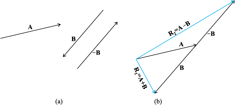
Fig. 3.5 (a) Two vectors A and B, – B is also shown. (b) Subtracting vector B from vector A – the result is R2. For comparison, addition of vectors A and B, i.e. R1 is also shown.
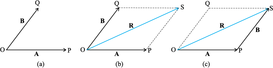
Fig. 3.6 (a) Two vectors A and B with their tails brought to a common origin. (b) The sum A + B obtained using the parallelogram method. (c) The parallelogram method of vector addition is equivalent to the triangle method.
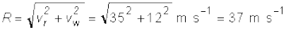
Example 3.1 Rain is falling vertically with a speed of 35 m s–1. Winds starts blowing after sometime with a speed of 12 m s–1 in east to west direction. In which direction should a boy waiting at a bus stop hold his umbrella?
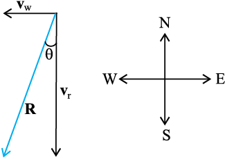
Fig. 3.7
Answer The velocity of the rain and the wind are represented by the vectors vr and vw in Fig. 3.7 and are in the direction specified by the problem. Using the rule of vector addition, we see that the resultant of vr and vw is R as shown in the figure. The magnitude of R is
The direction θ that R makes with the vertical is given by
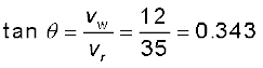
Or, 
Therefore, the boy should hold his umbrella in the vertical plane at an angle of about 19o with the vertical towards the east.
3.5 Resolution of vectors
Let a and b be any two non-zero vectors in a plane with different directions and let A be another vector in the same plane(Fig. 3.8). A can be expressed as a sum of two vectors — one obtained by multiplying a by a real number and the other obtained by multiplying b by another real number. To see this, let O and P be the tail and head of the vector A. Then, through O, draw a straight line parallel to a, and through P, a straight line parallel to b. Let them intersect at Q. Then, we have
A = OP = OQ + QP (3.6)
But since OQ is parallel to a, and QP is parallel to b, we can write :
OQ = λ a, and QP = µ b (3.7)
where λ and µ are real numbers.
Therefore, A = λ a + µ b (3.8)
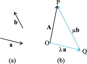
Fig. 3.8 (a) Two non-colinear vectors a and b.(b) Resolving a vector A in terms of vectors a and b.
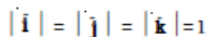
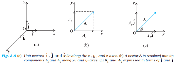
We say that A has been resolved into two component vectors λ a and µ b along a and b respectively. Using this method one can resolve a given vector into two component vectors along a set of two vectors – all the three lie in the same plane. It is convenient to resolve a general vector along the axes of a rectangular coordinate system using vectors of unit magnitude. These are called unit vectors that we discuss now. A unit vector is a vector of unit magnitude and points in a particular direction. It has no dimension and unit. It is used to specify a direction only. Unit vectors along the x-, y- and z-axes of a rectangular coordinate system are denoted by  ,
,  and
and  , respectively, as shown in Fig. 3.9(a).
Since these are unit vectors, we have
 (3.9)
(3.9)
These unit vectors are perpendicular to each other. In this text, they are printed in bold face with a cap (^) to distinguish them from other vectors. Since we are dealing with motion in two dimensions in this chapter, we require use of only two unit vectors. If we multiply a unit vector, say  by a scalar, the result is a vector
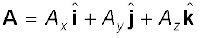
λ = λ . In general, a vector A can be written as
A = |A| (3.10)
where  is a unit vector along A.
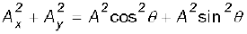
We can now resolve a vector A in terms of component vectors that lie along unit vectors  and
and  . Consider a vector A that lies in x-y plane as shown in Fig. 3.9(b). We draw lines from the head of A perpendicular to the coordinate axes as in Fig. 3.9(b), and get vectors A1 and A2 such that A1 + A2 = A. Since A1 is parallel to
  and A2 is parallel to
  , we have :
 , A2 = Ay
  (3.11)
where Ax and Ay are real numbers.
Thus, A = Ax  + Ay
+ Ay  (3.12)
This is represented in Fig. 3.9(c). The quantities Ax and Ay are called x-, and y- components of the vector A. Note that Ax is itself not a vector, but Ax  is a vector, and so is Ay
  . Using simple trigonometry, we can express Ax and Ay in terms of the magnitude of A and the angle θ it makes with the x-axis :
Ax = A cos θ
Ay = A sin θ (3.13)
As is clear from Eq. (3.13), a component of a vector can be positive, negative or zero depending on the value of θ.
Now, we have two ways to specify a vector A in a plane. It can be specified by :
(i) its magnitude A and the direction θ it makes with the x-axis; or
(ii) its components Ax and Ay
If A and θ are given, Ax and Ay can be obtained using Eq. (3.13). If Ax and Ay are given, A and θ can be obtained as follows :
 = A2
= A2
Or, 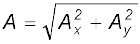 (4.14)
And 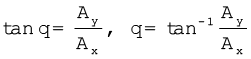 (4.15)
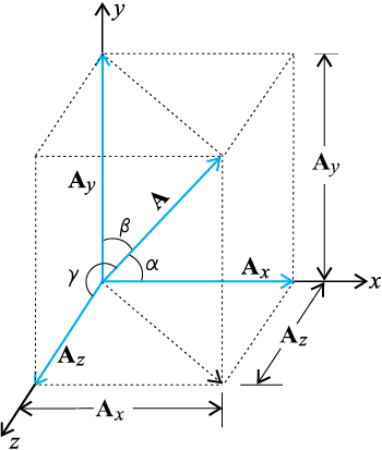
So far we have considered a vector lying in an x-y plane. The same procedure can be used to resolve a general vector A into three components along x-, y-, and z-axes in three dimensions. If α, β, and γ are the angles* between A and the x-, y-, and z-axes, respectively [Fig. 3.9(d)], we have
(d)
Fig. 3.9 (d) A vector A resolved into components along x-, y-, and z-axes
 (3.16a)
In general, we have
 (3.16b)
The magnitude of vector A is
 (3.16c)
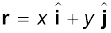
A position vector r can be expressed as
 (3.17)
where x, y, and z are the components of r along x-, y-, z-axes, respectively.
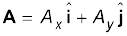
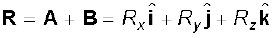
3.6 Vector addition – analytical method
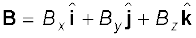
Although the graphical method of adding vectors helps us in visualising the vectors and the resultant vector, it is sometimes tedious and has limited accuracy. It is much easier to add vectors by combining their respective components. Consider two vectors A and B in x-y plane with components Ax, Ay and Bx, By :
 (3.18)
Let R be their sum. We have
R = A + B
 (3.19a)
Since vectors obey the commutative and associative laws, we can arrange and regroup the vectors in Eq. (4.19a) as convenient to us :
 (3.19b)
Since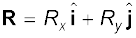 (3.20)
we have, 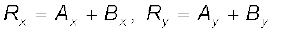 (3.21)
Thus, each component of the resultant vector R is the sum of the corresponding components of A and B.
In three dimensions, we have
with 
 (3.22)
This method can be extended to addition and subtraction of any number of vectors. For example, if vectors a, b and c are given as
 (3.23a)
then, a vector T = a + b – c has components :
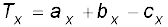
 (3.23b)
 .
.
Example 3.2 Find the magnitude and direction of the resultant of two vectors A and B in terms of their magnitudes and angle θ between them.
* Note that angles α, β, and γ are angles in space. They are between pairs of lines, which are not coplanar.
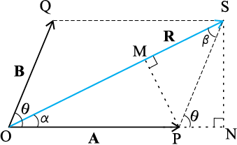
Fig. 3.10
Answer Let OP and OQ represent the two vectors A and B making an angle θ (Fig. 3.10). Then, using the parallelogram method of vector addition, OS represents the resultant vector R :
R = A + B
SN is normal to OP and PM is normal to OS.
From the geometry of the figure,
OS2 = ON2 + SN2
but ON = OP + PN = A + B cos θ SN = B sin θ
OS2 = (A + B cos θ)2 + (B sin θ)2
or, R2 = A2 + B2 + 2AB cos θ
 (3.24a)
In ∆ OSN, SN = OS sinα = R sinα, and in ∆ PSN, SN = PS sin θ = B sin θ
Therefore, R sin α = B sin θ
or,  (3.24b)
Similarly,
PM = A sin α = B sin β
or, 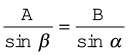 (3.24c)
Combining Eqs. (3.24b) and (3.24c), we get
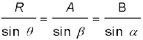 (3.24d)
Using Eq. (3.24d), we get:
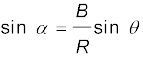 (3.24e)
where R is given by Eq. (3.24a).
or, 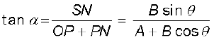 (3.24f)
Equation (3.24a) gives the magnitude of the resultant and Eqs. (3.24e) and (3.24f) its direction. Equation (3.24a) is known as the Law of cosines and Eq. (3.24d) as the Law of sines.
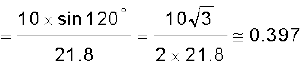
Example 3.3 A motorboat is racing towards north at 25 km/h and the water current in that region is 10 km/h in the direction of 60° east of south. Find the resultant velocity of the boat.
Answer The vector vb representing the velocity of the motorboat and the vector vc representing the water current are shown in Fig. 3.11 in directions specified by the problem. Using the parallelogram method of addition, the resultant R is obtained in the direction shown in the figure.
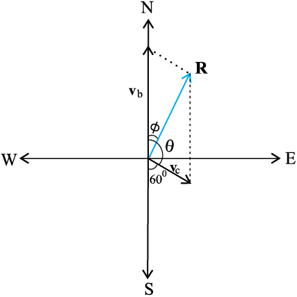
Fig. 3.11
We can obtain the magnitude of R using the Law of cosine :

To obtain the direction, we apply the Law of sines
 or,
or, 

3.7 Motion in a plane
In this section we shall see how to describe motion in two dimensions using vectors.
3.7.1 Position Vector and Displacement
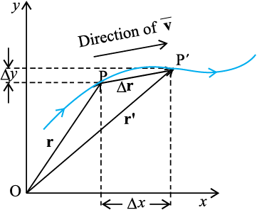
The position vector r of a particle P located in a plane with reference to the origin of an x-y reference frame (Fig. 3.12) is given by
where x and y are components of r along x-, and y- axes or simply they are the coordinates of the object.
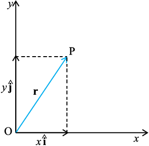
(a)
(b)
Fig. 3.12 (a) Position vector r. (b) Displacement ∆r and average velocity v of a particle.
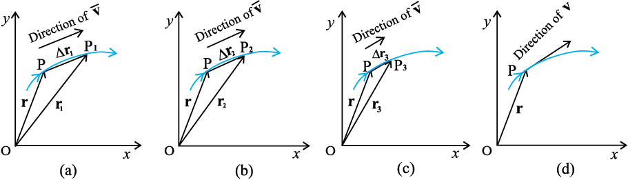
Fig. 3.13 As the time interval ∆t approaches zero, the average velocity approaches the velocity v. The direction of 3516.png is parallel to the line tangent to the path.
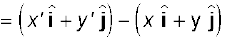
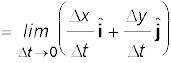
Suppose a particle moves along the curve shown by the thick line and is at P at time t and P′ at time t′ [Fig. 4.12(b)]. Then, the displacement is : ∆r = r′ – r (3.25)
and is directed from P to P′.
We can write Eq. (4.25) in a component form:
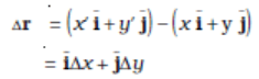
where ∆x = x ′ – x, ∆y = y′ – y (3.26)
Velocity
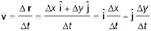
The average velocity of an object is the ratio of the displacement and the corresponding time interval :
 (3.27)
Or,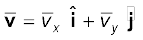
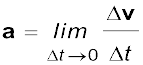
Since  , the direction of the average velocity is the same as that of ∆r (Fig. 3.12). The velocity (instantaneous velocity) is given by the limiting value of the average velocity as the time interval approaches zero :
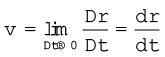 (3.28)
The meaning of the limiting process can be easily understood with the help of Fig 4.13(a) to (d). In these figures, the thick line represents the path of an object, which is at P at time t. P1, P2 and P3 represent the positions of the object after times ∆t1,∆t2, and ∆t3. ∆r1, ∆r2, and ∆r3 are the displacements of the object in times ∆t1, ∆t2, and ∆t3, respectively. The direction of the average velocity is shown in figures (a), (b) and (c) for three decreasing values of ∆t, i.e. ∆t1,∆t2, and ∆t3, (∆t1 > ∆t2 > ∆t3). As ∆t → 0, ∆r → 0
and is along the tangent to the path [Fig. 3.13(d)]. Therefore, the direction of velocity at any point on the path of an object is tangential to the path at that point and is in the direction of motion.

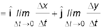 (3.29)
Or,
where . (3.30a)
So, if the expressions for the coordinates x and y are known as functions of time, we can use these equations to find vx and vy.
The magnitude of v is then
 (3.30b)
and the direction of v is given by the angle θ :
 (3.30c)
vx, vy and angle θ are shown in Fig. 3.14 for a velocity vector v at point p.
Acceleration
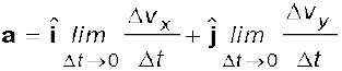
The average acceleration a of an object for a time interval ∆t moving in x-y plane is the change in velocity divided by the time interval :
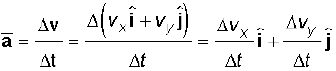 (3.31a)
Or, 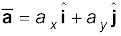 . (3.31b)
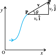
Fig. 3.14 The components vx and vy of velocity v and the angle θ it makes with x-axis. Note that vx = v cos θ, vy = v sin θ.
 (4.32a)
Since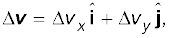 we have
Or,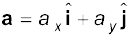 (4.32b)
where, 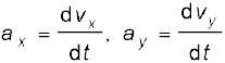 (4.32c)*
As in the case of velocity, we can understand graphically the limiting process used in defining acceleration on a graph showing the path of the object’s motion. This is shown in Figs. 3.15(a) to (d). P represents the position of the object at time t and P1, P2, P3 positions after time ∆t1, ∆t2, ∆t3, respectively (∆t 1> ∆t2>∆t3). The velocity vectors at points P, P1, P2, P3 are also shown in Figs. 3.15 (a), (b) and (c). In each case of ∆t, ∆v is obtained using the triangle law of vector addition. By definition, the direction of average acceleration is the same as that of ∆v. We see that as ∆t decreases, the direction of ∆v changes and consequently, the direction of the acceleration changes. Finally, in the limit ∆t 0 [Fig. 3.15(d)], the average acceleration becomes the instantaneous acceleration and has the direction as shown.
* In terms of x and y, ax and ay can be expressed as
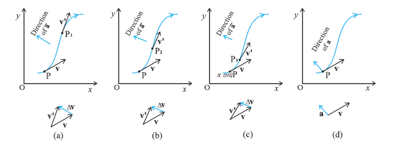
Fig. 3.15 The average acceleration for three time intervals (a) ∆t1, (b) ∆t2, and (c) ∆t3, (∆t1> ∆t2> ∆t3). (d) In the limit ∆t 0, the average acceleration becomes the acceleration.
Note that in one dimension, the velocity and the acceleration of an object are always along the same straight line (either in the same direction or in the opposite direction). However, for motion in two or three dimensions, velocity and acceleration vectors may have any angle between 0° and 180° between them.
Example 3.4 The position of a particle is given by where t is in seconds and the coefficients have the proper units for r to be in metres. (a) Find v(t) and a(t) of the particle. (b) Find the magnitude and direction of v(t) at t = 1.0 s.
Answer
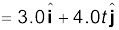
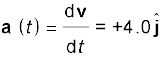
a = 4.0 m s–2 along y- direction
At t = 1.0 s,