
Chapter 4
Determinants
 All Mathematical truths are relative and conditional. — C.P. Steinmetz
4.1 Introduction
In the previous chapter, we have studied about matrices and algebra of matrices. We have also learnt that a system of algebraic equations can be expressed in the form of matrices. This means, a system of linear equations like

P.S. Laplace
(1749-1827)
a1 x + b1 y = c1
a2 x + b2 y = c2
can be represented as 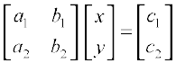 . Now, this system of equations has a unique solution or not, is determined by the number a1 b2 – a2 b1. (Recall that if
  or, a1 b2 – a2 b1 ≠ 0, then the system of linear equations has a unique solution). The number a1 b2 – a2 b1 which determines uniqueness of solution is associated with the matrix
 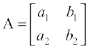 and is called the determinant of A or det A. Determinants have wide applications in Engineering, Science, Economics, Social Science, etc.
In this chapter, we shall study determinants up to order three only with real entries. Also, we will study various properties of determinants, minors, cofactors and applications of determinants in finding the area of a triangle, adjoint and inverse of a square matrix, consistency and inconsistency of system of linear equations and solution of linear equations in two or three variables using inverse of a matrix.
4.2 Determinant
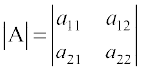
To every square matrix A = [aij] of order n, we can associate a number (real or complex) called determinant of the square matrix A, where aij = (i, j)th element of A. This may be thought of as a function which associates each square matrix with a unique number (real or complex). If M is the set of square matrices, K is the set of numbers (real or complex) and f : M → K is defined by f(A) = k, where A ∈ M and
k ∈ K, then f(A) is called the determinant of A. It is also denoted by |A| or det A or ∆.
If A =  , then determinant of A is written as |A| =
  = det (A)
Remarks
(i) For matrix A, |A| is read as determinant of A and not modulus of A.
(ii) Only square matrices have determinants.
4.2.1 Determinant of a matrix of order one
Let A = [a] be the matrix of order 1, then determinant of A is defined to be equal to a
4.2.2 Determinant of a matrix of order two
Let A = 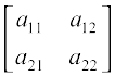 be a matrix of order 2 × 2,
then the determinant of A is defined as:
det (A) = |A| = ∆ = 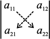 = a11a22 – a21a12
Example 1 Evaluate  .
.
Solution We have  = 2(2) – 4(–1) = 4 + 4 = 8.
Example 2 Evaluate 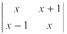
Solution We have
= x (x) – (x + 1) (x – 1) = x2 – (x2 – 1) = x2 – x2 + 1 = 1
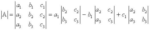
4.2.3 Determinant of a matrix of order 3 × 3
Determinant of a matrix of order three can be determined by expressing it in terms of second order determinants. This is known as expansion of a determinant along
a row (or a column). There are six ways of expanding a determinant of order
3 corresponding to each of three rows (R1, R2 and R3) and three columns (C1, C2 and C3) giving the same value as shown below.
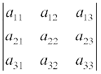
Consider the determinant of square matrix A = [aij]3 × 3
i.e., | A | = 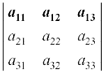
Expansion along first Row (R1)
Step 1 Multiply first element a11 of R1 by (–1)(1 + 1) [(–1)sum of suffixes in a11] and with the second order determinant obtained by deleting the elements of first row (R1) and first column (C1) of | A | as a11 lies in R1 and C1,
i.e., (–1)1 + 1 a11 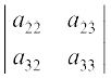
Step 2 Multiply 2nd element a12 of R1 by (–1)1 + 2 [(–1)sum of suffixes in a12] and the second order determinant obtained by deleting elements of first row (R1) and 2nd column (C2) of | A | as a12 lies in R1 and C2,
i.e., (–1)1 + 2 a12 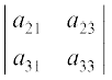
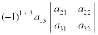
Step 3 Multiply third element a13 of R1 by (–1)1 + 3 [(–1)sum of suffixes in a13] and the second order determinant obtained by deleting elements of first row (R1) and third column (C3) of | A | as a13 lies in R1 and C3,
i.e., (–1)1 + 3 a13 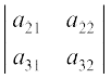
Step 4 Now the expansion of determinant of A, that is, | A | written as sum of all three terms obtained in steps 1, 2 and 3 above is given by
det A = |A| = (–1)1 + 1 a11 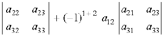
+ 
or |A| = a11 (a22 a33 – a32 a23) – a12 (a21 a33 – a31 a23)
+ a13 (a21 a32 – a31 a22)
= a11 a22 a33 – a11 a32 a23 – a12 a21 a33 + a12 a31 a23 + a13 a21 a32
– a13 a31 a22 ... (1)
Note We shall apply all four steps together.
Expansion along second row (R2)
| A | = 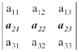
Expanding along R2, we get
| A | = 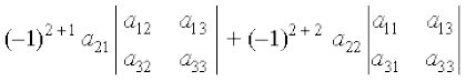
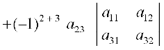
= – a21 (a12 a33 – a32 a13) + a22 (a11 a33 – a31 a13)
– a23 (a11 a32 – a31 a12)
| A | = – a21 a12 a33 + a21 a32 a13 + a22 a11 a33 – a22 a31 a13 – a23 a11 a32
+ a23 a31 a12
= a11 a22 a33 – a11 a23 a32 – a12 a21 a33 + a12 a23 a31 + a13 a21 a32
– a13 a31 a22 ... (2)
Expansion along first Column (C1)
| A | = 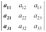
By expanding along C1, we get
| A | = 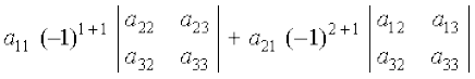
+ 
= a11 (a22 a33 – a23 a32) – a21 (a12 a33 – a13 a32) + a31 (a12 a23 – a13 a22)
| A | = a11 a22 a33 – a11 a23 a32 – a21 a12 a33 + a21 a13 a32 + a31 a12 a23
– a31 a13 a22
= a11 a22 a33 – a11 a23 a32 – a12 a21 a33 + a12 a23 a31 + a13 a21 a32
– a13 a31 a22 ... (3)
Clearly, values of |A| in (1), (2) and (3) are equal. It is left as an exercise to the reader to verify that the values of |A| by expanding along R3, C2 and C3 are equal to the value of |A| obtained in (1), (2) or (3).
Hence, expanding a determinant along any row or column gives same value.
Remarks
(i) For easier calculations, we shall expand the determinant along that row or column which contains maximum number of zeros.
(ii) While expanding, instead of multiplying by (–1)i + j, we can multiply by +1 or –1 according as (i + j) is even or odd.
(iii) Let A =  and B =
  . Then, it is easy to verify that A = 2B. Also |A| = 0 – 8 = – 8 and |B| = 0 – 2 = – 2.
Observe that, |A| = 4(– 2) = 22|B| or |A| = 2n|B|, where n = 2 is the order of square matrices A and B.
In general, if A = kB where A and B are square matrices of order n, then | A| = kn | B |, where n = 1, 2, 3
Example 3 Evaluate the determinant ∆ = 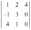 .
.
Solution Note that in the third column, two entries are zero. So expanding along third column (C3), we get
∆ = 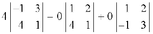
= 4 (–1 – 12) – 0 + 0 = – 52
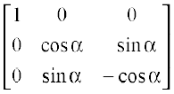
Example 4 Evaluate ∆ = 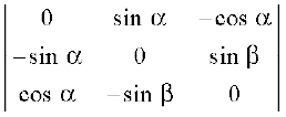 .
.
Solution Expanding along R1, we get
∆ = 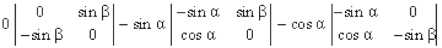
= 0 – sin α (0 – sin β cos α) – cos α (sin α sin β – 0)
= sin α sin β cos α – cos α sin α sin β = 0
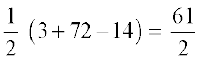
Example 5 Find values of x for which 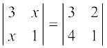 .
.
Solution We have
i.e. 3 – x2 = 3 – 8
i.e. x2 = 8
Hence x = ![]()
Exercise 4.1
Evaluate the determinants in Exercises 1 and 2.
1. 
2. (i) 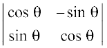 (ii)
(ii) 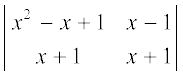
3. If A =  , then show that | 2A | = 4 | A |
4. If A =  , then show that | 3 A | = 27 | A |
5. Evaluate the determinants
(i)  (ii)
(ii) 
(iii)  (iv)
(iv) 
6. If A =  , find | A |
7. Find values of x, if
(i) 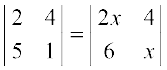 (ii)
(ii) 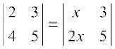
8. If 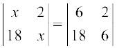 , then x is equal to
(A) 6 (B) ± 6 (C) – 6 (D) 0
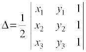
4.3 Area of a Triangle
In earlier classes, we have studied that the area of a triangle whose vertices are
(x1, y1), (x2, y2) and (x3, y3), is given by the expression ![]() [x1(y2–y3) + x2 (y3–y1) +
[x1(y2–y3) + x2 (y3–y1) +
x3 (y1–y2)]. Now this expression can be written in the form of a determinant as
∆ = 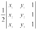 ... (1)
Remarks
(i) Since area is a positive quantity, we always take the absolute value of the determinant in (1).
(ii) If area is given, use both positive and negative values of the determinant for calculation.
(iii) The area of the triangle formed by three collinear points is zero.
Example 6 Find the area of the triangle whose vertices are (3, 8), (– 4, 2) and (5, 1).
Solution The area of triangle is given by
∆ = 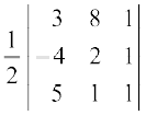
= 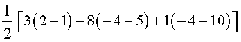
= 
Example 7 Find the equation of the line joining A(1, 3) and B (0, 0) using determinants and find k if D(k, 0) is a point such that area of triangle ABD is 3sq units.
Solution Let P (x, y) be any point on AB. Then, area of triangle ABP is zero (Why?). So
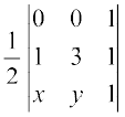 = 0
= 0
This gives 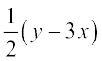 = 0 or y = 3x,
which is the equation of required line AB.
Also, since the area of the triangle ABD is 3 sq. units, we have
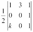 = ± 3
= ± 3
This gives,  , i.e., k = ± 2
Exercise 4.2
1. Find area of the triangle with vertices at the point given in each of the following :
(i) (1, 0), (6, 0), (4, 3) (ii) (2, 7), (1, 1), (10, 8)
(iii) (–2, –3), (3, 2), (–1, –8)
2. Show that points
A (a, b + c), B (b, c + a), C (c, a + b) are collinear.
3. Find values of k if area of triangle is 4 sq. units and vertices are
(i) (k, 0), (4, 0), (0, 2) (ii) (–2, 0), (0, 4), (0, k)
4. (i) Find equation of line joining (1, 2) and (3, 6) using determinants.
(ii) Find equation of line joining (3, 1) and (9, 3) using determinants.
5. If area of triangle is 35 sq units with vertices (2, – 6), (5, 4) and (k, 4). Then k is
(A) 12 (B) –2 (C) –12, –2 (D) 12, –2
4.4 Minors and Cofactors
In this section, we will learn to write the expansion of a determinant in compact form using minors and cofactors.
Definition 1
Minor of an element aij of a determinant is the determinant obtained by deleting its ith row and jth column in which element aij lies. Minor of an element aij is denoted by Mij.
Remark
Minor of an element of a determinant of order n(n ≥ 2) is a determinant of order n – 1.
Example 8 Find the minor of element 6 in the determinant 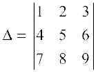
Solution Since 6 lies in the second row and third column, its minor M23 is given by
M23 =  = 8 – 14 = – 6 (obtained by deleting R2 and C3 in ∆).
Definition 2 Cofactor of an element aij, denoted by Aij is defined by
Aij = (–1)i + j Mij, where Mij is minor of aij.
Example 9 Find minors and cofactors of all the elements of the determinant 
Solution Minor of the element aij is Mij
Here a11 = 1. So M11 = Minor of a11= 3
M12 = Minor of the element a12 = 4
M21 = Minor of the element a21 = –2
M22 = Minor of the element a22 = 1
Now, cofactor of aij is Aij. So
A11 = (–1)1 + 1 M11 = (–1)2 (3) = 3
A12 = (–1)1 + 2 M12 = (–1)3 (4) = – 4
A21 = (–1)2 + 1 M21 = (–1)3 (–2) = 2
A22 = (–1)2 + 2 M22 = (–1)4 (1) = 1
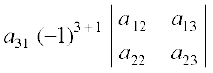
Example 10 Find minors and cofactors of the elements a11, a21 in the determinant
∆ = 
Solution By definition of minors and cofactors, we have
Minor of a11 = M11 =  = a22 a33– a23 a32
Cofactor of a11 = A11 = (–1)1+1 M11 = a22 a33 – a23 a32
Minor of a21 = M21 =  = a12 a33 – a13 a32
Cofactor of a21 = A21 = (–1)2+1 M21 = (–1) (a12 a33 – a13 a32) = – a12 a33 + a13 a32
Remark Expanding the determinant ∆, in Example 21, along R1, we have
∆ = (–1)1+1 a11 + (–1)1+2 a12  + (–1)1+3 a13
= a11 A11 + a12 A12 + a13 A13, where Aij is cofactor of aij
= sum of product of elements of R1 with their corresponding cofactors
Similarly, ∆ can be calculated by other five ways of expansion that is along R2, R3, C1, C2 and C3.
Hence ∆ = sum of the product of elements of any row (or column) with their corresponding cofactors.
Note If elements of a row (or column) are multiplied with cofactors of any other row (or column), then their sum is zero. For example,
∆ = a11 A21 + a12 A22 + a13 A23
= a11 (–1)1+1 + a12 (–1)1+2  + a13 (–1)1+3
=  = 0 (since R1 and R2 are identical)
Similarly, we can try for other rows and columns.
Example 11 Find minors and cofactors of the elements of the determinant
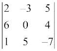 and verify that a11 A31 + a12 A32 + a13 A33= 0
Solution We have M11 =  = 0 –20 = –20; A11 = (–1)1+1 (–20) = –20
M12 =  = – 42 – 4 = – 46; A12 = (–1)1+2 (– 46) = 46
M13 =  = 30 – 0 = 30; A13 = (–1)1+3 (30) = 30
M21 =  = 21 – 25 = – 4; A21 = (–1)2+1 (– 4) = 4
M22 =  = –14 – 5 = –19; A22 = (–1)2+2 (–19) = –19
M23 =  = 10 + 3 = 13; A23 = (–1)2+3 (13) = –13
M31 =  = –12 – 0 = –12; A31 = (–1)3+1 (–12) = –12
M32 =  = 8 – 30 = –22; A32 = (–1)3+2 (–22) = 22
and M33 =  = 0 + 18 = 18; A33 = (–1)3+3 (18) = 18
Now a11 = 2, a12 = –3, a13 = 5; A31 = –12, A32 = 22, A33 = 18
So a11 A31 + a12 A32 + a13 A33
= 2 (–12) + (–3) (22) + 5 (18) = –24 – 66 + 90 = 0
Exercise 4.3
Write Minors and Cofactors of the elements of following determinants:
1. (i)  (ii)
(ii) 
2. (i)  (ii)
(ii) 
3. Using Cofactors of elements of second row, evaluate ∆ = 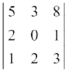 .
.
4. Using Cofactors of elements of third column, evaluate ∆ = 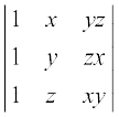 .
.
5. If ∆ = and Aij is Cofactors of aij, then value of ∆ is given by
(A) a11 A31+ a12 A32 + a13 A33 (B) a11 A11+ a12 A21 + a13 A31
(C) a21 A11+ a22 A12 + a23 A13 (D) a11 A11+ a21 A21 + a31 A31
4.5 Adjoint and Inverse of a Matrix
In the previous chapter, we have studied inverse of a matrix. In this section, we shall discuss the condition for existence of inverse of a matrix.
To find inverse of a matrix A, i.e., A–1 we shall first define adjoint of a matrix.
4.6.1 Adjoint of a matrix
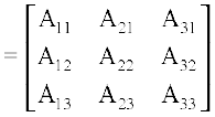
Definition 3 The adjoint of a square matrix A = [aij]n × n is defined as the transpose of the matrix [Aij]n × n, where Aij is the cofactor of the element aij. Adjoint of the matrix A is denoted by adj A.
Let 
Then 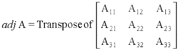
Example 12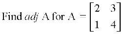
Solution We have A11 = 4, A12 = –1, A21 = –3, A22 = 2
Hence adj A = 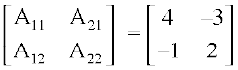
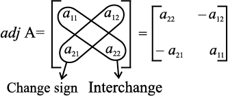
Remark For a square matrix of order 2, given by
A = 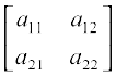
The adj A can also be obtained by interchanging a11 and a22 and by changing signs of a12 and a21, i.e.,
We state the following theorem without proof.
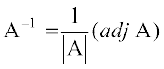
Theorem 1 If A be any given square matrix of order n, then
A(adj A) = (adj A) A = ![]() ,
,
where I is the identity matrix of order n
Verification
Let A =  , then adj A =
Since sum of product of elements of a row (or a column) with corresponding cofactors is equal to |A| and otherwise zero, we have
A (adj A) = 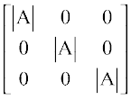 =
= ![]()
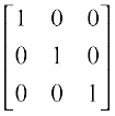 =
= ![]() I
I
Similarly, we can show (adj A) A = ![]() I
I
Hence A (adj A) = (adj A) A = ![]() I
I
Definition 4 A square matrix A is said to be singular if ![]() = 0.
= 0.
For example, the determinant of matrix A =  is zero
Hence A is a singular matrix.
Definition 5 A square matrix A is said to be non-singular if ![]() ≠ 0
≠ 0
Let A =  . Then
 ![]() =
=  = 4 – 6 = – 2 ≠ 0.
Hence A is a nonsingular matrix
We state the following theorems without proof.
Theorem 2 If A and B are nonsingular matrices of the same order, then AB and BA are also nonsingular matrices of the same order.
Theorem 3 The determinant of the product of matrices is equal to product of their respective determinants, that is, ![]() =
= ![]()
![]() , where A and B are square matrices of the same order
, where A and B are square matrices of the same order
Remark We know that (adj A) A = ![]() I =
I = 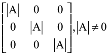
Writing determinants of matrices on both sides, we have
![]() =
= 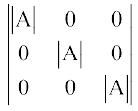
i.e. |(adj A)| |A| = 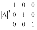 (Why?)
i.e. |(adj A)| |A| = |A|3 (1)
i.e. |(adj A)| = |A|2
In general, if A is a square matrix of order n, then |adj(A)| = |A|n – 1.
Theorem 4 A square matrix A is invertible if and only if A is nonsingular matrix.
Proof Let A be invertible matrix of order n and I be the identity matrix of order n.
Then, there exists a square matrix B of order n such that AB = BA = I
Now AB = I. So ![]() =
= ![]() or
or ![]()
![]() = 1
= 1 ![]()
This gives ![]() ≠ 0. Hence A is nonsingular.
≠ 0. Hence A is nonsingular.
Conversely, let A be nonsingular. Then ![]() ≠ 0
≠ 0
Now A (adj A) = (adj A) A = ![]() I (Theorem 1)
I (Theorem 1)
or A 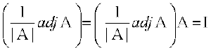
or AB = BA = I, where B = 
Thus A is invertible and A–1 =
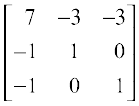
Example 13 If A = 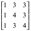 , then verify that A adj A = |A| I. Also find A–1.
Solution We have ![]() = 1 (16 – 9) –3 (4 – 3) + 3 (3 – 4) = 1 ≠ 0
= 1 (16 – 9) –3 (4 – 3) + 3 (3 – 4) = 1 ≠ 0
Now A11 = 7, A12 = –1, A13 = –1, A21 = –3, A22 = 1, A23 = 0, A31 = –3, A32 = 0, A33 = 1
Therefore adj A = 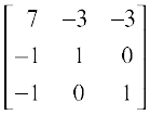
Now A (adj A) = 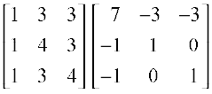
= 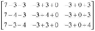
= = (1) = ![]() . I
. I
Also A–1 =
= 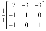 =
= 
Example 14 If A = 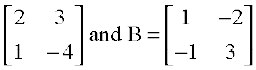 , then verify that (AB)–1 = B–1A–1.
Solution We have AB = 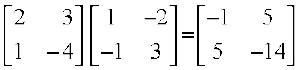
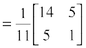
Since, ![]() = –11 ≠ 0, (AB)–1 exists and is given by
= –11 ≠ 0, (AB)–1 exists and is given by
(AB)–1 = 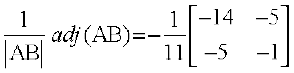
Further, ![]() = –11 ≠ 0 and
= –11 ≠ 0 and ![]() = 1 ≠ 0. Therefore, A–1 and B–1 both exist and are given by
= 1 ≠ 0. Therefore, A–1 and B–1 both exist and are given by
A–1 = 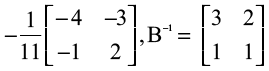
Therefore 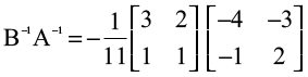
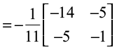
Hence (AB)–1 = B–1 A–1
Example 15 Show that the matrix A =  satisfies the equation A2 – 4A + I = O, where I is 2 × 2 identity matrix and O is 2 × 2 zero matrix. Using this equation, find A–1.
Solution We have 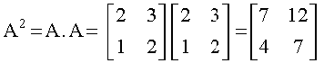
Hence 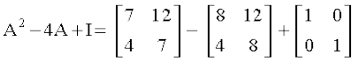
Now A2 – 4A + I = O
Therefore A A – 4A = – I
or A A (A–1) – 4 A A–1 = – I A–1 (Post multiplying by A–1 because |A| ≠ 0)
or A (A A–1) – 4I = – A–1
or AI – 4I = – A–1
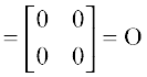
or A–1 = 4I – A = 
Hence 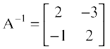
Exercise 4.4
Find adjoint of each of the matrices in Exercises 1 and 2.
1. 
2. 
Verify A (adj A) = (adj A) A = |A| I in Exercises 3 and 4
3. 
4. 
Find the inverse of each of the matrices (if it exists) given in Exercises 5 to 11.
5. 
6. 
7. 
8. 
9. 
10. 
11. 
12. Let A =  and B =
  . Verify that (AB)–1 = B–1 A–1.
13. If A =  , show that A2 – 5A + 7I = O. Hence find A–1.
14. For the matrix A =  , find the numbers a and b such that A2 + aA + bI = O.
15. For the matrix A = 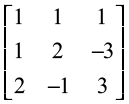
Show that A3– 6A2 + 5A + 11 I = O. Hence, find A–1.
16. If A = 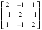
Verify that A3 – 6A2 + 9A – 4I = O and hence find A–1
17. Let A be a nonsingular square matrix of order 3 × 3. Then |adj A| is equal to
(A) |A| (B) |A|2 (C) |A|3 (D) 3|A|
18. If A is an invertible matrix of order 2, then det (A–1) is equal to
(A) det (A) (B)  (C) 1 (D) 0
4.6 Applications of Determinants and Matrices
In this section, we shall discuss application of determinants and matrices for solving the system of linear equations in two or three variables and for checking the consistency of the system of linear equations.
Consistent system A system of equations is said to be consistent if its solution (one or more) exists.
Inconsistent system A system of equations is said to be inconsistent if its solution does not exist.
Note In this chapter, we restrict ourselves to the system of linear equations having unique solutions only.
4.6.1 Solution of system of linear equations using inverse of a matrix
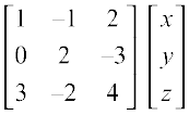
Let us express the system of linear equations as matrix equations and solve them using inverse of the coefficient matrix.
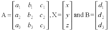
Consider the system of equations
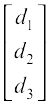
a1 x + b1 y + c1 z = d1
a2 x + b2 y + c2 z = d2
a3 x + b3 y + c3 z = d3
Let A = 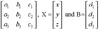
Then, the system of equations can be written as, AX = B, i.e.,
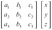 =
= 
Case I If A is a nonsingular matrix, then its inverse exists. Now
AX = B
or A–1 (AX) = A–1 B (premultiplying by A–1)
or (A–1A) X = A–1 B (by associative property)
or I X = A–1 B
or X = A–1 B
This matrix equation provides unique solution for the given system of equations as inverse of a matrix is unique. This method of solving system of equations is known as Matrix Method.
Case II If A is a singular matrix, then |A| = 0.
In this case, we calculate (adj A) B.
If (adj A) B ≠ O, (O being zero matrix), then solution does not exist and the system of equations is called inconsistent.
If (adj A) B = O, then system may be either consistent or inconsistent according as the system have either infinitely many solutions or no solution.
Example 16 Solve the system of equations
2x + 5y = 1
3x + 2y = 7
Solution The system of equations can be written in the form AX = B, where
A = 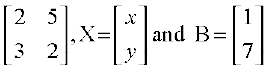
Now, ![]() = –11 ≠ 0, Hence, A is nonsingular matrix and so has a unique solution.
= –11 ≠ 0, Hence, A is nonsingular matrix and so has a unique solution.
Note that A–1 = 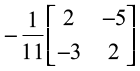
Therefore X = A–1B = – 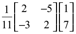
i.e. ![]() =
= 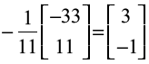
Hence x = 3, y = – 1
Example 17 Solve the following system of equations by matrix method.
3x – 2y + 3z = 8
2x + y – z = 1
4x – 3y + 2z = 4
Solution The system of equations can be written in the form AX = B, where
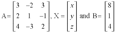
We see that
![]() = 3 (2 – 3) + 2(4 + 4) + 3 (– 6 – 4) = – 17 ≠ 0
= 3 (2 – 3) + 2(4 + 4) + 3 (– 6 – 4) = – 17 ≠ 0
Hence, A is nonsingular and so its inverse exists. Now
A11 = –1, A12 = – 8, A13 = –10
A21 = –5, A22 = – 6, A23 = 1
A31 = –1, A32 = 9, A33 = 7
Therefore A–1 = 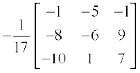
So X = 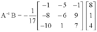
i.e. ![]() =
= 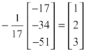
Hence x = 1, y = 2 and z = 3.
Example 18 The sum of three numbers is 6. If we multiply third number by 3 and add second number to it, we get 11. By adding first and third numbers, we get double of the second number. Represent it algebraically and find the numbers using matrix method.
Solution Let first, second and third numbers be denoted by x, y and z, respectively. Then, according to given conditions, we have
x + y + z = 6
y + 3z = 11
x + z = 2y or x – 2y + z = 0
This system can be written as A X = B, where
A = 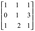 , X =
, X = ![]() and B =
and B = ![]()
Here ![]() . Now we find adj A
. Now we find adj A
A11 = 1 (1 + 6) = 7, A12 = – (0 – 3) = 3, A13 = – 1
A21 = – (1 + 2) = – 3, A22 = 0, A23 = – (– 2 – 1) = 3
A31 = (3 – 1) = 2, A32 = – (3 – 0) = – 3, A33 = (1 – 0) = 1
Hence adj A = 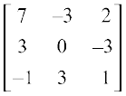
Thus A –1 = ![]() adj (A) =
adj (A) = 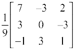
Since X = A–1 B
X = 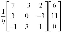
or ![]() =
= ![]()
 =
= ![]()
 =
= ![]()
Thus x = 1, y = 2, z = 3
Exercise 4.5
Examine the consistency of the system of equations in Exercises 1 to 6.
1. x + 2y = 2
2x + 3y = 3
2. 2x – y = 5
x + y = 4
3. x + 3y = 5
2x + 6y = 8
4. x + y + z = 1
2x + 3y + 2z = 2
ax + ay + 2az = 4
5. 3x–y – 2z = 2
2y – z = –1
3x – 5y = 3
6. 5x – y + 4z = 5
2x + 3y + 5z = 2
5x – 2y + 6z = –1
Solve system of linear equations, using matrix method, in Exercises 7 to 14.
7. 5x + 2y = 4
7x + 3y = 5
8. 2x – y = –2
3x + 4y = 3
9. 4x – 3y = 3
3x – 5y = 7
10. 5x + 2y = 3
3x + 2y = 5
11. 2x + y + z = 1
x – 2y – z = ![]()
12. x – y + z = 4
2x + y – 3z = 0
x + y + z = 2
3x – y – 2z = 3
13. 2x + 3y +3 z = 5
x – 2y + z = – 4
14. x – y + 2z = 7
3x + 4y – 5z = – 5
2x – y + 3z = 12
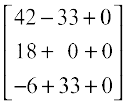
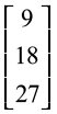
15. If A =  , find A–1. Using A–1 solve the system of equations
2x – 3y + 5z = 11
3x + 2y – 4z = – 5
x + y – 2z = – 3
16. The cost of 4 kg onion, 3 kg wheat and 2 kg rice is ₹ 60. The cost of 2 kg onion, 4 kg wheat and 6 kg rice is ₹90. The cost of 6 kg onion 2 kg wheat and 3 kg rice is ₹ 70. Find cost of each item per kg by matrix method.
Miscellaneous Examples
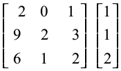
Example 19 Use product 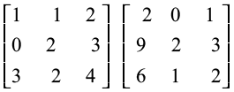 to solve the system of equations
x – y + 2z = 1
2y – 3z = 1
3x – 2y + 4z = 2
Solution Consider the product 
= 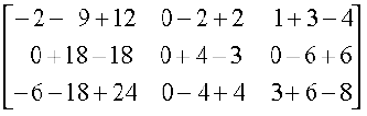 =
= 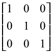
Hence 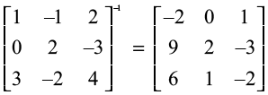
Now, given system of equations can be written, in matrix form, as follows
 =
= ![]()
or ![]() =
= 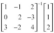 =
= 
= 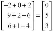
Hence x = 0, y = 5 and z = 3
Miscellaneous Exercises on Chapter 4
1. Prove that the determinant 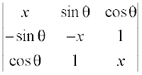 is independent of θ.
2. Evaluate  .
.
3. If A–1 - = 
4. Let A =  . Verify that
(i) [adj A]–1 = adj (A–1) (ii) (A–1)–1 = A
5. Evaluate 
6. Evaluate 
Using properties of determinants in Exercises 11 to 15, prove that:
7. Solve the system of equations

Choose the correct answer in Exercise 17 to 19.
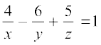
8. If x, y, z are nonzero real numbers, then the inverse of matrix 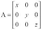 is
is
(A) 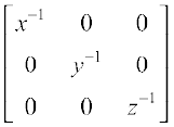 (B)
(B) 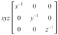
(C) 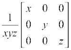 (D)
(D) 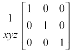
9. Let A = 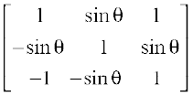 , where 0 ≤ θ ≤ 2π. Then
(A) Det(A) = 0 (B) Det(A) ∈ (2, ∞)
(C) Det(A) ∈ (2, 4) (D) Det(A) ∈ [2, 4]
Summary
![]() Determinant of a matrix A = [a11]1×1 is given by |a11| = a11
Determinant of a matrix A = [a11]1×1 is given by |a11| = a11
![]() Determinant of a matrix
Determinant of a matrix 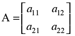 is given by
 = a11 a22 – a12 a21
![]() Determinant of a matrix
Determinant of a matrix  is given by (expanding along R1)
For any square matrix A, the |A| satisfy following properties.
![]() Area of a triangle with vertices (x1, y1), (x2, y2) and (x3, y3) is given by
Area of a triangle with vertices (x1, y1), (x2, y2) and (x3, y3) is given by
![]() Minor of an element aij of the determinant of matrix A is the determinant obtained by deleting ith row and jth column and denoted by Mij.
Minor of an element aij of the determinant of matrix A is the determinant obtained by deleting ith row and jth column and denoted by Mij.
![]() Cofactor of aij of given by Aij = (– 1)i+j Mij
Cofactor of aij of given by Aij = (– 1)i+j Mij
![]() Value of determinant of a matrix A is obtained by sum of product of elements of a row (or a column) with corresponding cofactors. For example,
Value of determinant of a matrix A is obtained by sum of product of elements of a row (or a column) with corresponding cofactors. For example,
![]() = a11 A11 + a12 A12 + a13 A13.
= a11 A11 + a12 A12 + a13 A13.
![]() If elements of one row (or column) are multiplied with cofactors of elements of any other row (or column), then their sum is zero. For example, a11 A21 + a12 A22 + a13 A23 = 0
If elements of one row (or column) are multiplied with cofactors of elements of any other row (or column), then their sum is zero. For example, a11 A21 + a12 A22 + a13 A23 = 0
![]() If
If 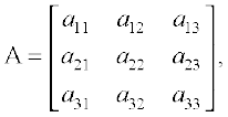 then
then 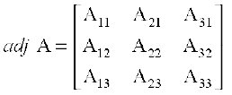 , where Aij is cofactor of aij
![]() A (adj A) = (adj A) A = |A| I, where A is square matrix of order n.
A (adj A) = (adj A) A = |A| I, where A is square matrix of order n.
![]() A square matrix A is said to be singular or non-singular according as
A square matrix A is said to be singular or non-singular according as
|A| = 0 or |A| ≠ 0.
![]() If AB = BA = I, where B is square matrix, then B is called inverse of A.
If AB = BA = I, where B is square matrix, then B is called inverse of A.
Also A–1 = B or B–1 = A and hence (A–1)–1 = A.
![]() A square matrix A has inverse if and only if A is non-singular.
A square matrix A has inverse if and only if A is non-singular.
![]()
![]() If a1 x + b1 y + c1 z = d1
If a1 x + b1 y + c1 z = d1
a2 x + b2 y + c2 z = d2
a3 x + b3 y + c3 z = d3,
then these equations can be written as A X = B, where
![]() Unique solution of equation AX = B is given by X = A–1 B, where
Unique solution of equation AX = B is given by X = A–1 B, where ![]() .
.
![]() A system of equation is consistent or inconsistent according as its solution exists or not.
A system of equation is consistent or inconsistent according as its solution exists or not.
![]() For a square matrix A in matrix equation AX = B
For a square matrix A in matrix equation AX = B
(i) |A| ≠ 0, there exists unique solution
(ii) |A| = 0 and (adj A) B ≠ 0, then there exists no solution
(iii) |A| = 0 and (adj A) B = 0, then system may or may not be consistent.
Historical Note
The Chinese method of representing the coefficients of the unknowns of several linear equations by using rods on a calculating board naturally led to the discovery of simple method of elimination. The arrangement of rods was precisely that of the numbers in a determinant. The Chinese, therefore, early developed the idea of subtracting columns and rows as in simplification of a determinant
Mikami, China, pp 30, 93.
Seki Kowa, the greatest of the Japanese Mathematicians of seventeenth century in his work ‘Kai Fukudai no Ho’ in 1683 showed that he had the idea of determinants and of their expansion. But he used this device only in eliminating a quantity from two equations and not directly in the solution of a set of simultaneous linear equations. T. Hayashi, “The Fakudoi and Determinants in Japanese Mathematics,” in the proc. of the Tokyo Math. Soc., V.
Vendermonde was the first to recognise determinants as independent functions. He may be called the formal founder. Laplace (1772), gave general method of expanding a determinant in terms of its complementary minors. In 1773 Lagrange treated determinants of the second and third orders and used them for purpose other than the solution of equations. In 1801, Gauss used determinants in his theory of numbers.
The next great contributor was Jacques - Philippe - Marie Binet, (1812) who stated the theorem relating to the product of two matrices of m-columns and n-rows, which for the special case of m = n reduces to the multiplication theorem.
Also on the same day, Cauchy (1812) presented one on the same subject. He used the word ‘determinant’ in its present sense. He gave the proof of multiplication theorem more satisfactory than Binet’s.
The greatest contributor to the theory was Carl Gustav Jacob Jacobi, after this the word determinant received its final acceptance.